Whither cosmic rays?

NOTE: This page uses MathJax, a JavaScript program running in your web browser, to render equations. It renders the equations in three steps: 1. during loading you may see the “raw code” that generates the equations, 2. an HTML version of the equations is pre-rendered (functional, but not nice looking), then 3. a full and proper “typeset” rendering of the equations. Depending on the speed of your system and browser, it may take a few seconds to tens of seconds to finish the whole process. The end product is usually worth the wait, imho.

This is the next instalment in Phelonius’ Pedantic Solutions which aims to tackle something I wish I had when I was doing my physics degree: some step-by-step solutions to problems that explained how each piece was done in a painfully clear way (sometimes I was pretty thick and missed important points that are maybe obvious to me now, looking back). I have realized I could have benefited from a more integrated approach to examples, where whatever tools that are needed are explained as the solution is presented, so that is at the core of these attempts. I have also been told all my life that the best way to learn something is to try to teach it to someone else, and so this is part of my attempt to become more agile and comfortable with the ideas and tools needed to do modern physics. If you don’t understand something, please ask, because I haven’t explained it well enough and others will surely be confused as well.

Things covered:

  • Cosmic rays and detectors
  • Probability Density Functions (PDFs)
  • Cumulative Distribution Functions (CDFs)
  • Inverting functions
  • Monte-Carlo simulations
  • Geometric and trigonometric identity proofs
  • You were probably lied to

Cosmic rays have always fascinated me. I had the chance, once upon a time, to work on a scientific payload proposal for a student-run CubeSat satellite design (part of the 1st Canadian Satellite Design Challenge), and I jumped at the chance. What I present here is part of that effort. I had previously worked on three cosmic ray experiments as an undergraduate (with my electronics and software development experience mostly… I am still but a larval physicist): two versions of a system that used naturally occurring cosmic rays to produce tomographic images of whatever was inside (3D images like a CT scan), and another to observe changes in the intensity and direction of cosmic rays using a solar weather observatory I mostly built (I had to move, 6 bricks at a time on a hand truck, 2.4 metric tonnes of lead as shielding from another building across campus, ugh, worst summer job ever but the results were worth it).

As part of the satellite payload design, I built a proof-of-concept cosmic ray detector out of mostly scrap I was able to scrounge together (and a few basic supplies I had to buy). The cosmic ray detector consisted of two 1/2″ thick, 15cm x 15cm plastic scintillator panels instrumented with photomultiplier (PMT) tubes. Every time an ionizing particle goes through one of the scintillator panels, it gives off a trail of photons, some of which hit the face of the PMTs which are sensitive enough to pick up single photons and generate an electrical pulse in response. These panels were separated by 1.0m and had 15cm of lead bricks between them. Note: the lead bricks block any local radiation from radioactive sources in the environment, but most cosmic rays pass right through them. If the PMT on only one scintillator is activated, that event is ignored (either it was noise from the PMT, local radiation not powerful enough to go through the lead, or a cosmic ray that didn’t go through both panels because of its path); but if it goes through both scintillators (and the lead between them and fires both associated PMTs), then that event is counted.

Un-normalized cos^2(x)

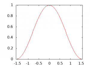
So here’s the problem… I needed to know how many cosmic rays to expect to pass through both scintillator panels of my detector. Once I knew that, I could compare that with the number I actually got from the experimental apparatus, and that would let me know how good the scrap detector I had built was. There is an excellent free resource on cosmic ray physics (and so much other physics) in the Particle Data Group’s “Review of Particle Physics”. The whole thing is here, but the sub-section on cosmic ray physics is here (note, this link is to a PDF document). As an aside, you can order a print copy of this massive publication for free no matter where you live (or download the whole thing as a PDF), it’s pretty boffo. Here’s the tl;dr version for this solution: if you hold your thumb nail horizontally, about one cosmic ray passes through your thumbnail (and every other part of your body) every minute… the rate is about 1 per square centimetre per minute (and they are mostly made of muons and their energy is 3GeV on average if that’s of any use to you). Cosmic rays mostly come from directly overhead, but they can be from any direction of the sky and follow, roughly, a \(cos^{2}(\theta)\) probability distribution (see diagram, note that the x-axis is from \(-\pi/2\) through \(\pi/2\), but expressed as a decimal number). This means that the relative probability of a cosmic ray coming from any particular angle relative to directly upwards can be calculated by plugging that angle into \(cos^{2}(\theta)\), e.g. at \(\theta = 0\) radians (\(0^\circ\)) from vertical, \(cos^{2}(0) = 1\); but at \(\theta = \pi/3\) radians (\(60^\circ\)) from vertical (\(\pi/6 = 30^\circ\) up from from the horizon), there’s a 75% smaller chance of a cosmic ray from that angle since \(cos^{2}(\pi/3) = 0.25\).

This all comes back to the detector in trying to figure out what percentage of the cosmic rays hitting the top scintillator also hit the bottom panel (did I mention I stood it on its side so that one scintillator panel was directly above the other one?). Since the panels are 15cm x 15cm, I would expect roughly (very roughly) 225 cosmic rays per minute (15cm x 15cm x 1 cosmic ray per square centimetre per minute) to hit the upper surface of the top panel, which is very roughly about 4 per second. But only those cosmic rays that go through both scintillator panels is counted as an “event”. I tried to calculate what’s called the solid-angle acceptance of the detector for the given angular distribution of cosmic rays, but my brain broke and it looked like trying to calculate it directly was way more trouble than it was worth (if you have a way of doing this, please share your solution, it got nasty pretty quick for me).

An easier way to tackle this kind of problem is to write a Monte Carlo simulation (named after a city renowned for its gambling, and thus its association with random numbers). I’ll perhaps go into the nitty gritty another time, but in this case it involves randomly and uniformly picking an X/Y coordinate for the cosmic ray to pass through the top scintillator panel (the cosmic ray is equally likely to pass through any point on its surface), a uniformly distributed random direction to come from relative to the horizontal (a \(2\pi\) radians = 360° circle, think degrees from north), and then randomly picking the angle (relative to vertical) the cosmic ray came from to hit that X/Y location. The trick with the last part is that computers are really good at picking uniform random numbers (where any random value is as likely as any other random value within the range they are being generated over), but they don’t tend to have the ability to pick a random number according to any other non-uniform probability function. To make this work then, I needed to figure out a way of converting from a uniform random number into a \(cos^{2}(\theta)\) distribution. I learned how to do this in a 4th year Computational Physics course (PHYS4807 at Carleton University in Ottawa, Canada) that was a triple-headed monster in that it taught C++ (I was good there, most were not), complex statistical methods as used in advanced particle physics in the real world (the first time any of us had seen anything that complex in terms of statistical analysis), and did it using the ROOT scientific computing program from CERN (which nobody knew). Note: ROOT is free to download and use, is an incredibly powerful scientific computing framework, and is used by ATLAS and other experiments at CERN to do analysis.

Once I had a simulated cosmic ray passing through the top panel (at a particular point, from a particular direction, at a particular angle relative to the vertical), I calculated whether it would hit the bottom panel if it continued in a straight line (not a bad assumption for cosmic rays, fyi). If it did, then I counted it as an event. By doing random generation of virtual cosmic ray events, I just had to run the simulation long enough to get a very accurate estimation of what percentage of cosmic rays hitting the top panel went through both panels. Since I knew from observed physics how often a particle should hit the top panel, and then “observing” the percentage of those that passed through both panels from the simulation, I would be able to estimate the number cosmic ray events in my real detector and see if my real measurements were close at all.

The process of allowing the computer to generate an arbitrary (non-uniform) random distribution consists of three phases:

  • Determine the Probability Density Function (PDF)
  • Calculate the Cumulative Distribution Function (CDF) from the PDF
  • Invert the CDF to get the formula

The equation derived in the last step is what is used to convert from a uniform distribution like computer-generated random numbers into the distribution specified by the PDF, which is \(cos^{2}(\theta)\) in this case.

We know already that the relative probability of a cosmic ray coming from any particular angle off of vertical is \(cos^{2}(\theta)\) (from experimental results, sort of… that is a simplification but good enough for this application). But how to convert that into a proper PDF? The key is the notion of “probability”, and specifically if a cosmic ray is observed it had to come from somewhere (some angle). When the relative probabilities are added up for every possible angle, we need to get 100% (again, it just says that all events came from some angle, so the probabilities all add up to 1 = 100%). Since the angle, \(\theta\), is a continuous variable (it is a real number), when we integrate the PDF over its angular range the solution must be 1. This process is called normalization (so the probability of an observed cosmic ray coming from somewhere is 100%). The function \(cos^{2}(\theta)\) is unnormalized since taking its integral from \(-\pi/2\) to \(\pi/2\) results in a value greater than 1 (a probability greater than 100% is a nonsensical concept). To normalize the PDF, a normalization constant is put into the probability function (I use \(A\) in this case), then that constant is calculated by doing the integral (to which we know the solution we must get). Note that sometimes the normalization constant could be 1, but it may not be obvious before doing the integration, so the integration required to do the normalization is generally a required step. The normalized PDF has the following form:

\[ f(\theta) = A\cdot cos^{2}(\theta)\tag{1} \]

Remember that if \(f(\theta) = A\cdot cos^{2}(\theta)\), then \(f(\diamond) = A\cdot cos^{2}(\diamond)\) since \(\theta\) is just a symbol and can be replaced with anything as long as the new symbol is carried through the whole equation. To fully determine the PDF, we need to figure out the value of \(A\) in the following (I’ll talk about the \(\theta’\) stuff below).

\[ \int_{\theta’ = -\pi/2}^{\theta’ = \pi/2} f(\theta’)\, d\theta’ = \int_{-\pi/2}^{\pi/2} A\cdot cos^{2}(\theta’)\, d\theta’ = 1\tag{2} \]

where the range of the integral, \(-\pi/2\) through \(\pi/2\) just provides a \(\pi\) radians (180°) range from horizon to horizon with \(\theta = 0\) being directly overhead. Again, it is equal to \(1\) because once all the probabilities are added up (integrated in this case), the result must be 100%. Cosmic rays don’t travel through the Earth very far, so they generally don’t come from below the horizon in any significant number. I could have limited the angular range of the integral even further because of the geometry of my detector (two detector panels, one above the other), but I wanted to make a generic “cosmic ray generator” that I could use in other applications. Conversely, if I needed to generate a very large number of potential cosmic ray events, it would save computing power to have tailored the simulation to my specific detector. That was not necessary here: it’s a small detector, there are relatively few events, and I have lots of idle computing power on my desk.

Why the \(\theta’\) in the integrals? Well, it’s not strictly needed here because there would be no confusion between the integration variable (sometimes called the dummy variable) and the actual variable we care about (which is what specifies the limits on the integral). However, if there is an actual variable in the limits, which often happens and there will be when we calculate the CDF, there can be confusion about what is the integration variable and what is a limit if there is no way to glance at the equation and tell (it’s usually possible to figure out from context, but it just increases the chances of a mistake). As I have said in previous posts, the integration variable is irrelevant because it gets replaced with the limits during the evaluation phase and just disappears. This whole idea of “priming” integration variables (using it as a dummy variable) is common but really confused the heck out of me when I was learning. Now that I have (mostly) figured out why it is done, I just think of it in an abstract way. For instance, I could just as easily have written it with \(\oplus\) instead of \(\theta’\), and we would get the exact same answer at the end:

\[ \int_{\oplus = -\pi/2}^{\oplus = \pi/2} f(\oplus)\, d\oplus = \int_{-\pi/2}^{\pi/2} A\cdot cos^{2}(\oplus)\, d\oplus = 1\tag{2} \]

The reason for putting primes on the variable that underlies the calculation is that it helps remember what the equation is about, but also reminds us that it’s just an integration (aka dummy) variable. If we’re calculating stuff related to angles, then \(\theta’\) reminds us of that. Something like \(\oplus\) does the job (and explicitly reminds us that it’s a dummy variable), but it is completely abstract and provides no hint as to what we’re working with. Every scrap of information and/or structure can potentially help when working on a problem, so it is best not to deliberately toss any away if it can be helped. To that end, when I’m using \(\theta\) (or anything) as an integration variable, I will try to remember to put a “prime” on it here, but will continue to simply use \(\theta\) when I’m talking about angles.

It’s easy to integrate \(cos(\theta)\), but \(cos^{2}(\theta) = cos(\theta)\cdot cos(\theta)\)? That integral is hard to solve as-is (yeah, it can be looked up in a table or solved online, but the idea here is to solve it ourselves). Is there any way to get rid of the squared trigonometric function? The answer is yes, but it’s non-obvious in that you’re only likely to know about it if you’ve seen the necessary trigonometric identity before. I will derive that identity below since it’s good practice (and is a bit of an art form), but here’s the spoiler:

\[\int_{-\pi/2}^{\pi/2} A\cdot cos^{2}(\theta’)\, d\theta’ = \int_{-\pi/2}^{\pi/2} A\cdot \frac{1 + cos(2\theta’)}{2} d\theta’ = 1 \]

This integral is quite easy to do because the \(1/2\) and \(A\) can be brought outside the integral since they are both constant, and the remaining piece can be broken into the sum of two integrals because integration is a linear operator (more on this below).

Trigonometric Identity Proofs Helper

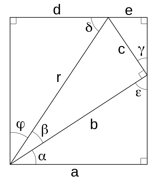
The diagram here can be used to prove the two common trigonometric identities that I needed to derive the other identity I used in solving this integral (there are so many ways to solve the integral, this was the one that came to mind for me). On the diagram, lengths are labelled with roman letters and angles are labelled with greek letters. Trigonometric identities are simply some statement about trigonometry is equal to some other statement about trigonometry, and they are usually derived by using other known properties of trigonometry. The fewer the assumptions, the more fundamental the identity; however, new identities are built out of more fundamental ones that have been proven, so answers to trigonometric questions can be answered with rigorous proofs using identities that have already themselves been rigorously proven. It can be quite fun to do this, but it can also be crazy-making if the path forward is not obvious. This is one of the branches of math where artistry and intuition, along with experience and a command of many techniques, is required to get solutions. There is no such thing in deriving identities as “plug and chug” solutions, and each requires some degree of insight.

Two assumptions that will be used in the proofs are the definitions of the sine and cosine functions. A quick reminder of another definition though: a right triangle is a triangle that has one of its angles as \(\pi/2\) radians (90°), a right angle. The sine of one of the non-right angles in a right triangle is the ratio of the length of the side opposite that angle divided by the length of the hypotenuse (the side opposite the right angle). The cosine of one of the non-right angles in a right triangle is the ratio of the length of the non-hypotenuse side adjacent to the angle divided by the length of the hypotenuse. The other assumption used in one of the proofs is the Pythagorean theorem that states that the square of the length of the hypotenuse is equal to the sum of the squares of the lengths of both other sides. Using the off-kilter right angle triangle in the middle of the rectangle here, these can be expressed mathematically as:

\[ sin(\beta) = \frac{c}{r}\ \ \ \ \ \ cos(\beta) = \frac{b}{r}\ \ \ \ \ \ r^{2} = b^{2} + c^{2} \]

The first necessary identity is one I have seen used just about everywhere, and it has to do with squared trigonometric functions (like we’re dealing with). Looking at the right triangle inside the rectangle whose sides are of length \(b\), \(c\), and \(r\):

\[ sin(\beta) = \frac{c}{r}\,\rightarrow\, c = r\cdot sin(\beta)\ \ \ \ \ \ cos(\beta) = \frac{b}{r}\,\rightarrow\, b = r\cdot cos(\beta) \]

Using the Pythagorean theorem and substituting the above:

\[ r^{2} = b^{2} + c^{2}\,\rightarrow\, r^{2} = \left(r\cdot cos(\beta)\right)^{2} + \left(r\cdot sin(\beta)\right)^{2} \]

Doing the squares, dividing it all by \(r^{2}\), and re-arranging slightly:

\[ \frac{r^{2}}{r^{2}} = \frac{r^{2}\cdot cos^{2}(\beta)}{r^{2}} + \frac{r^{2}\cdot sin^{2}(\beta)}{r^{2}}\,\rightarrow\, cos^{2}(\beta) + sin^{2}(\beta) = 1 \]

Which is the standard form of this important trigonometric identity. Solving for the value we are dealing with in the integral, we get:

\[ cos^{2}(\beta) = 1\, – sin^{2}(\beta)\tag{3} \]

We still have a \(sin^{2}(\beta)\) so it may not look like we’re any further ahead, but there’s another identity that will allow us to get rid of it, which I will derive now. This proof, including the diagram above, is based on an excellent video presentation by Linda Green titled “Proof of the Angle Sum Formula” [1]. We will need the solutions for the lengths of right triangle sides \(b\) and \(c\) relative to angle \(\beta\) from above. We also need the following observations about various labelled angles. Recall that the angles of any triangle on a plane (flat surface) always add up to \(\pi\) radians (180°), and that a right angle is \(\pi / 2\) radians (90°). We get:

\[ \epsilon = \pi – \frac{\pi}{2} – \alpha = \frac{\pi}{2} – \alpha \]

which is just the total sum of the angles of the triangle, \(\pi\), minus the right angle, \(\pi/2\), minus the other angle in the triangle, \(\alpha\), and leaves the size of the angle \(\epsilon\). Similarly:

\[ \gamma = \pi – \frac{\pi}{2}\, – \epsilon = \frac{\pi}{2}\, – \epsilon = \frac{\pi}{2}\, – \left(\frac{\pi}{2}\, – \alpha\right) = \frac{\pi}{2}\, – \frac{\pi}{2} + \alpha = \alpha \]

Here it’s done a little differently in that we know that the angle \(\epsilon\) plus the angle \(\gamma\) plus the right angle, \(\pi/2\), sandwiched between them add up to \(\pi\) because they add up to a straight line (which is \(\pi\) radians, 180°). Then we can observe that (with some substitution, re-arranging, and remembering we have shown that \(\gamma = \alpha\)):

\[ sin(\gamma) = sin(\alpha) = \frac{e}{c}\,\rightarrow\, e = c\cdot sin(\alpha) = [r\cdot sin(\beta))]\cdot sin(\alpha) = r\cdot sin(\alpha)\cdot sin(\beta) \]

\[ cos(\alpha) = \frac{a}{b}\,\rightarrow\, a = b\cdot cos(\alpha) = [r\cdot cos(\beta)]\cdot cos(\alpha) = r\cdot cos(\alpha)\cdot cos(\beta) \]

Following the same sort of logic:

\[ \psi = \frac{\pi}{2}\, – \alpha\, – \beta \]

\[ \delta = \pi\, – \frac{\pi}{2}\, – \psi = \frac{\pi}{2}\, – \left(\frac{\pi}{2}\, – \alpha\, – \beta\right) = \frac{\pi}{2}\, – \frac{\pi}{2} + \alpha + \beta = \alpha + \beta \]

Then:

\[ cos(\delta) = cos(\alpha + \beta) = \frac{d}{r}\,\rightarrow\, d = r\cdot cos(\alpha + \beta) \]

Since the line \(d e\) is parallel with line \(a\) (i.e. \(de \parallel a\)), and they are the same length since they are opposite sides of a rectangle, then substituting:

\[ a = d + e\,\rightarrow\, r\cdot cos(\alpha)\cdot cos(\beta) = r\cdot cos(\alpha + \beta) + r\cdot sin(\alpha)\cdot sin(\beta) \]

Then dividing both sides by \(r\) and re-arranging:

\[ cos(\alpha + \beta) = cos(\alpha)\cdot cos(\beta)\, – sin(\alpha)\cdot sin(\beta)\tag{4} \]

Which is the second standard identity we needed to derive. As indicated above, this one is the “sum of angles” identity. If we let \(\alpha = \beta = \theta\), then \(\alpha + \beta = 2\theta\) , and we get:

\[ cos(\alpha + \beta) = cos(\theta + \theta) = cos(\theta)\cdot cos(\theta)\, – sin(\theta)\cdot sin(\theta) \]

And so,

\[ cos(2\theta) = cos^{2}(\theta)\, – sin^{2}(\theta)\,\rightarrow\, sin^{2}(\theta) = cos^{2}(\theta)\, – cos(2\theta)\tag{5} \]

And we have an identity that defines \(sin^{2}(\theta)\) with respect to \(cos^{2}(\theta)\) and \(cos(2\theta)\) (the latter of which is what we want because it is not a squared trigonometric function). And then the fun part where it all sorts itself out, substituting equation (5) into equation (3):

\[ cos^{2}(\theta) = 1\, – sin^{2}(\theta) = 1\, – \left(cos^{2}(\theta)\, – cos(2\theta)\right) = 1\, – cos^{2}(\theta) + cos(2\theta) \]

Then re-arranging:

\[ 2\cdot cos^{2}(\theta) = 1 + cos(2\theta)\,\rightarrow\, cos^{2}(\theta) = \frac{1 + cos(2\theta)}{2} \]

And there we have the identity we need to use to solve the integral for the PDF. Again, while it was possible to just look it up, one of the problems I had in my undergraduate degree is I was given too much “plug and play” math and didn’t get to do any proper mathematical proofs until I was in my 3rd year (and then only because I took an Abstract Algebra elective), and this really caused problems in my 4th years studies where I really needed to understand where the math I was using came from (and how it could be derived). So heading back to the integral of the PDF function:

\[ \int_{-\pi/2}^{\pi/2} A\cdot cos^{2}(\theta’)\, d\theta’ = \int_{-\pi/2}^{\pi/2} A\cdot \frac{1 + cos(2\theta’)}{2}\, d\theta’ = 1 \]

This can be re-written as (bringing the constants to the front):

\[ \frac{A}{2} \int_{-\pi/2}^{\pi/2} \left[1 + cos(2\theta’)\right]\, d\theta’ = \frac{A}{2} \left[\int_{-\pi/2}^{\pi/2} 1\, d\theta’ + \int_{-\pi/2}^{\pi/2} cos(2\theta’)\, d\theta’\right] = 1 \]

We know that the integral of a sum is the sum of the integrals because integration is a linear function (see “Decay and Growth Rates” for more information on this property of integration). We don’t know how to solve the integral of \(cos(2\theta)\), but we do know how to do \(cos(\theta)\) (or \(cos(u)\), which is what will be used), so we can use the substitution technique to tackle this integral. But first, let’s solve the first of the two integrals to get it out of the way:

\[ \int_{-\pi/2}^{\pi/2} 1\, d\theta’ = \int_{-\pi/2}^{\pi/2} \theta’^{\, 0}\, d\theta’ = \frac{1}{0 + 1}\left.\theta’^{\, 0 + 1}\right|_{-\pi/2}^{\pi/2} = \left.\theta’\right|_{-\pi/2}^{\pi/2} = \left(\frac{\pi}{2}\right)\, -\left(-\frac{\pi}{2}\right) = \pi \]

So,

\[ \frac{A}{2} \left[\pi + \int_{\theta’ = -\pi/2}^{\theta’ = \pi/2} cos(2\theta’)\, d\theta’\right] = 1\tag{6} \]

To solve the remaining integral with the substitution method, let \(u = 2\theta’\), therefore:

\[ \frac{du}{d\theta’} = \frac{d}{d\theta’}(2\theta’) = 2\,\rightarrow\, d\theta’ = \frac{du}{2} \]

(if you didn’t understand what just happened, check out “Relativistic energy expansion” ). Now to substitute: a process that has to be done carefully and completely. Looking at the above, we can see that the infinitesimal \(d\theta’\) should be replaced with \(du/2\), and that \(2\theta’ = u\). What is often confusing with the substitution method (at least for me as I was learning) is that the limits of the integral also need to be converted to the new variable (\(\theta’ \rightarrow u\) in this case), which is why I explicitly reminded myself in equation (6) that the limits are specified as \(\theta’\). To convert from \(\theta’\) to \(u\), we have specified \(u = 2\theta’\), so for the upper limit (\(\theta’ = \pi/2\)), \(u = 2\theta’ = 2(\pi/2) = \pi\). Similarly, for the lower limit (\(\theta’ = -\pi/2\)), \(u = 2\theta’ = 2(-\pi/2) =\, -\pi\). The converted function is then:

\[ \frac{A}{2} \left[\pi + \int_{u = -\pi}^{u = \pi} cos(u)\, \frac{du}{2}\right] = \frac{A}{2} \left[\pi + \frac{1}{2}\int_{-\pi}^{\pi} cos(u)\, du\right] = 1 \]

which is an integral that is trivial to do:

\[ \frac{A}{2} \left[\pi + \frac{1}{2}\left.sin(u)\right|_{u = -\pi}^{u = \pi}\right] = \frac{A}{2} \left[\pi + \left(sin(\pi)\, – sin(-\pi)\right)\right] = 1 \]
\[= \frac{A}{2} \left[\pi + \left(0\, – 0\right)\right] = \frac{A\pi}{2} = 1\,\rightarrow\, A = \frac{2}{\pi} \]

Since there is no \(u\) in the value calculated for \(A\), it does not need to be converted back to the variable \(\theta\). Now that we have our normalization constant, substituting it into equation (1) allows us to fully specify the PDF:

\[ f(\theta) = \frac{2}{\pi}\cdot cos^{2}(\theta)\tag{7} \]

Normalized cos^2(x)

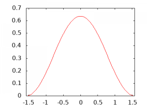
The normalized PDF is shown in the diagram. Note that the only difference is that the peak at \(\theta = 0\) is just lower, but the shape is the same. Somewhat of a slog but hopefully a straightforward one, this is about as easy as integrals get. The next part is also straightforward in terms of math (it’s just a few steps), but it took me a long time to wrap my brain around what was going on. To generate the Cumulative Distribution Function (CDF), you integrate the PDF. The integral starts at the same lower limit; however, instead of using \(\pi/2\) as the upper limit, you use the PDF variable instead (\(\theta\) in this case). What this does is allows some value of \(\theta\) to be plugged into the solved equation, and the answer will be the cumulative integral to that point.

\[ F(\theta) = \int_{\theta’=-\pi/2}^{\theta’=\theta} f(\theta’)\,d\theta’ = \int_{-\pi/2}^{\theta} f(\theta’)\,d\theta’ \]

I specify the overall function, \(F\), as a function of the variable \(\theta\) because the result will be dependent on what value we choose for that variable (it is specified as one of the limits rather as an integration/dummy variable, which is \(\theta’\)). We know from doing the PDF that \(-\pi/2 \leq \theta \leq \pi/2\). We also know that if we integrate over the full range (i.e. setting \(\theta = \pi/2\) when evaluating the integral), we get the answer as 1 (since we normalized the PDF). I hope it is clear that if we set \(\theta =\, -\pi/2\), then the answer of the integral will be 0 (since we’re not actually integrating over any range). Therefore, the possible values of the solution over the range of possible values for \(\theta\) is such that \(0 \leq F(\theta) \leq 1\) because of the way we’ve constructed the PDF so the probabilities over its range will integrate to 100%. Jumping ahead again, if you haven’t realized already, this is how to get the result we are after: if we choose a \(\theta\) and evaluate the integral, we get a number between 0 and 1 inclusive. The computer can generate a random number between 0 and 1, so if we set that as the solution, then we can invert the function and determine which \(\theta\) would give that answer. Because we are using the CDF to do this, the resulting distribution of probabilities will match the \(cos^{2}(\theta)\) distribution we need!

Note that I put primes on the variables involved with the integration part (and left the variables involved with the evaluation part unprimed). This is a reminder that it doesn’t matter what symbol is used when doing an integral, it’s the limits that remain in the solution after they are substituted in after the integration is done.

But first, we need to solve the CDF. We let the solution be \(r\), which represents the “forward” direction for the solution where we specify \(\theta\) and solve for \(r\), but which will be turned backwards after we get a solution so we can specify \(r\) and solve for \(\theta\) (which is called, fittingly, inverting the equation).

\[ F(\theta) = \int_{-\pi/2}^{\theta} f(\theta’)\, d\theta’ = \int_{-\pi/2}^{\theta}\frac{2}{\pi}\cdot cos^{2}(\theta’)\, d\theta’ = r \]

\[ \frac{\pi r}{2} = \int_{-\pi/2}^{\theta}cos^{2}(\theta’)\, d\theta’ = \int_{-\pi/2}^{\theta} \frac{1 + cos(2\theta’)}{2}\, d\theta’ = \frac{1}{2}\int_{-\pi/2}^{\theta} \left[1 + cos(2\theta’)\right]\, d\theta’ \]

Multiplying both sides by 2 and using the linear property of integration:

\[ \pi r = \int_{-\pi/2}^{\theta} 1\, d\theta’ + \int_{-\pi/2}^{\theta} cos(2\theta’)\, d\theta’ = \int_{-\pi/2}^{\theta} d\theta’ + \int_{-\pi/2}^{\theta} cos(2\theta’)\, d\theta’ \]

Solving the leftmost integral and doing the substitution \(u = 2\theta\):

\[ \pi r = \left.\theta’\right|_{-\pi/2}^{\theta} + \frac{1}{2}\int_{-\pi}^{2\theta} cos(u)\, du = \theta\, – \left(-\frac{\pi}{2}\right) + \frac{1}{2}\cdot \left. sin(u)\right|_{-\pi}^{2\theta} \]

\[ = \theta + \frac{\pi}{2} + \frac{1}{2}\left[ sin(2\theta)\, – sin(-\pi) \right] = \theta + \frac{\pi}{2} + \frac{1}{2}\left[ sin(2\theta)\, – 0 \right] \]

Multiplying both sides by 2, simplifying, and re-arranging:

\[ 2\pi r = 2\theta + \pi + sin(2\theta)\,\rightarrow\, 2\pi r\, – \pi = 2\theta + sin(2\theta)\tag{8} \]

Which is our CDF. If we pick a value for \(\theta\), we can use the following equation to easily get an answer for \(r\) between 0 and 1:

\[ r(\theta) = \frac{2\theta + sin(2\theta) + \pi}{2\pi}\tag{9} \]

Giving it a try, for \(\theta = -\pi/2\), \(\theta = \pi/2\), and \(\theta = 0\):

\[ r(\theta = -\pi/2) = \frac{2\cdot(-\pi/2) + sin(2\cdot(-\pi/2)) + \pi}{2\pi} = \frac{-\pi + sin(-\pi) + \pi}{2\pi} = \frac{0}{2\pi} = 0 \]

\[ r(\theta = \pi/2) = \frac{2\cdot(\pi/2) + sin(2\cdot(\pi/2)) + \pi}{2\pi} = \frac{\pi + sin(\pi) + \pi}{2\pi} = \frac{2\pi}{2\pi} = 1 \]

\[ r(\theta = 0) = \frac{2\cdot 0 + sin(2\cdot 0) + \pi}{2\pi} = \frac{0 + sin(0) + \pi}{2\pi} = \frac{\pi}{2\pi} = \frac{1}{2} = 0.5 \]

All of which are the expected answers, so this looks good. Note that the answer \(0.5\) was expected for \(\theta = 0\) because the \(cos^2(\theta)\) function is symmetric around \(\theta = 0\), so integrating it from \(-\pi/2\) to \(0\) will give the same answer as integrating from \(0\) to \(\pi/2\). Therefore integrating to \(0\) will give \(1/2\) of the answer of integrating to \(\pi/2\) (which gives 1).

Lovely. Now, let’s switch it around so if we provide an \(r\) between 0 and 1, we can solve for the \(\theta\) that gives that result. Now here’s one of the reasons why I am doing these solutions: I was lied to. Lied to big time! You might even be in the same position. You see, likely out of necessity and without malice (I hope), all the problems provided to me (and maybe you) as part of my undergraduate degree had analytic solutions (meaning you can you use mathematical symbol manipulation to get an answer). Here, in a process that took many weeks of me thinking I did something wrong with my solutions (repeating the derivation a half-dozen times and getting the same result), or that I was missing some key tool in solving for \(\theta\) in this very simple equation, I discovered the ugly truth: there is no way to solve this equation using any known analytic mathematical technique (or nothing anyone would admit to)! When I went hat in hand for help to a professor I knew, they glanced at it and said “oh, there’s no solution, you’ll have to solve it numerically”. All of the work I did as an undergraduate had not prepared me for this revelation. In fact, most problems can only be solved using either approximation methods, or numerically (hopefully using a computer). I say lie, but it’s more of a lie by omission rather than a direct falsehood (nobody ever told me that all problems could be solved), but it meant I had reached the limits of human knowledge trying to invert what looked to me like a trivial equation. Humbling.

The good news is there are lots of programs that will take an equation with two variables, a value for one of the variables, and can then solve for the other variable numerically. One such package is ROOT, which I mentioned earlier, and was what I had planned to use for my simulation framework anyway. Implementing it in ROOT is not terribly difficult if you know where to look and how to use it. Your mileage may vary, as the saying goes, but it can certainly be learned. Getting a feel for numerically solving this equation is not hard because it can be done with WolframAlpha online. To do it, just enter Equation (9), but instead of using the variable \(r\), you need to specify a number between 0 and 1 inclusive in its place (I also used the variable \(x\) because it’s easier to type, it doesn’t make any difference). The line to type for \(r = 1\) is:

(2 x + Sin[2 x] + Pi)/(2 Pi) == 1

For \(r = 0\):

(2 x + Sin[2 x] + Pi)/(2 Pi) == 0

For \(r = 0.5\):

(2 x + Sin[2 x] + Pi)/(2 Pi) == 0.5

And so on. I ran those in that order and got the answers \(\pi/2\), \(-\pi/2\), and \(0\) respectively (in the section “Solution:” near the bottom of the web page for me). If you are feeling particularly keen to see if it generates a \(cos^2(\theta)\) distribution, you can use the following to generate a random \(r\) and a random \(\theta\) (or \(x\) in this case) from it:

(2 x + Sin[2 x] + Pi)/(2 Pi) == RandomReal[]

You can build a histogram using \(x\) (or \(\theta\)) as your x-axis, dividing up the range (between say \(-1.6\) and \(+1.6\)) into “bins”, and increasing each bin count by one any time the result from the above code falls within that bin. With enough samples, even plotting it by hand on a piece of paper, you will eventually see the \(cos^2(\theta)\) shape taking form. If you do a very large numbers of samples (using a loop and a computer program hopefully), it makes a very nice \(2/\pi\cdot cos^2(\theta)\) distribution. I did this myself with a ROOT program (many tens of thousands of samples) and then overlaid the actual \(2/\pi\cdot cos^2(\theta)\) function, and it was a perfect match. This let me know I wasn’t completely out to lunch on this technique.

CDF of cos^2(x)

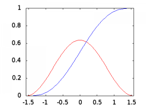
The last question is then: how does this work? If you look at the plot of the CDF over its range from \(-\pi/2\) to \(\pi/2\) (plotted on the x-axis), you can see how the CDF (in blue) increases as we increase the angle towards \(\pi/2\). Each point on the plot is the result from Equation (9), where \(F(\theta)\) (plotted on the y-axis) is calculated for each \(\theta\) value. Comparing it to the normalized PDF (in red), you can see how there’s not much area to integrate on its left, so the CDF increases slowly; but near the middle the PDF is at its maximum and so is the rate of increase of the CDF. Once past \(\theta = 0\), the PDF starts to decrease its height, so the rate of increase of the CDF decreases as it approaches 1 as there is again less to integrate.

Remember that instead of calculating \(0 \leq F(\theta) \leq 1\) when given a \(\theta\) where \(-\pi/2 \leq \theta \leq \pi/2\), we want to calculate \(-\pi/2 \leq \theta \leq \pi/2\) given a \(0 \leq F(\theta) \leq 1\) (which we call \(r\) to remember that we’re randomly generating this number between 0 and 1 inclusive). So, if you look at the CDF plot (in blue), imagine picking a random number between 0 and 1 and drawing a horizontal line across the plot at that y-axis value. Where that line intersects the blue CDF plot line, you draw a vertical line down to the x-axis and that will give you a \(\theta\) value between \(-\pi/2\) and \(\pi/2\) inclusive. But, it’s way easier to “hit” the CDF plot with a horizontal when its slope is high (“hitting the broad side of a barn”, it presents a much larger “target” to horizontal lines from the y-axis along its middle section); but when its slope is lower (e.g. at the bottom and top), there are many fewer chances to hit that section of the plot with a horizontal line if they are randomly distributed along the y-axis (and any \(r\) number has an equal chance of being selected). Because the horizontal lines in the middle of the 0 to 1 range have a higher chance of “hitting” the CDF plot, the chances of an “event” towards the middle of the angular range is much greater. The opposite is true at the edges of the plot. When you generate enough events, their random distribution is uniform in \(r\) but will follow a \(cos^2\) distribution in \(\theta\). And so, using this \(\theta\) distribution will give us the angular distribution we want for our simulated cosmic rays and we have the tricky part for our Monte Carlo simulation ready to roll.

To run the cosmic ray simulation then, I wrote a loop that generated 4 uniform random numbers every pass (each between 0 and 1, with each number equally probable). The first and second were multiplied by 15cm to figure out where the virtual cosmic ray would pass through the upper detector panel (an X coordinate and a Y coordinate). I subtracted 7.5cm from each of the coordinates so the (X,Y) = (0,0) point was in the middle of the upper detector (it made a later calculation easier). The third number was multiplied by \(2\pi\) radians to figure out which compass direction the virtual cosmic ray was coming from. And the fourth number was fed into an equation solver to generate the angle from vertical as a number between \(-\pi/2\) and \(\pi/2\). The four numbers fully specified the trajectory of the cosmic ray through the upper detector panel. Since cosmic rays are so energetic and penetrating (they generally pass through my detector material without hitting any atoms, and bounce off course very little if they do), I just had to project its trajectory in a straight line and figure out what it’s (X,Y) coordinate would be when it intersected the plane of the bottom detector panel (1.0m below the top panel). This was done with basic trigonometry. If the (X,Y) coordinates were each within 7.5cm of the centre of the panel in both X and Y directions, then it was logged as a coincident event (a hit in both panels). From this, I could get a ratio of coincident hits in the detector vs. total cosmic rays hitting the top panel (and would then let me get an expected coincidence count). Running the simulation long enough, I got a good average expected number of coincident cosmic ray events per unit of time. The actual number of physical coincident events I measured in my detector was sufficiently lower than the simulated number that I know that my detector isn’t super duper, but it was still good enough to do the work I wanted to do.

If you have any feedback, or questions, please leave a comment so others can see it. I will try to answer if I can. If you think this was valuable to you, please leave a comment or send me an email at to dafriar23@gmail.com. If you want to use this in some way yourself (other than for personal use to learn), please contact me at the given email address and we’ll see what we can do.

© 2019 James Botte. All rights reserved.

P.S. I used gnuplot running on a CentOS 7 Linux system for the plots. This is the code I used for the last plot:

set yrange[0:1]
set xrange[-pi/2:pi/2]
set terminal png size 400,300
set output 'output.png'
set multiplot
plot 2/pi * cos(x) * cos(x) lt rgb "red"
plot (2*x + sin(2*x) + pi)/(2 * pi) lt rgb "blue"
unset multiplot

Note: When setting the “terminal” to output to PNG image format, gnuplot on my system output (just fyi in case you try and the font looks different):

Options are 'nocrop font "/usr/share/fonts/dejavu/DejaVuSans.ttf,12" fontscale 1.0 size 400,300'

Posted in Mathematics, Pedantic, Physics | Leave a comment

This pressure needs to let up a little…

NOTE: This page uses MathJax, a JavaScript program running in your web browser, to render equations. It renders the equations in three steps: 1. during loading you may see the “raw code” that generates the equations, 2. an HTML version of the equations is pre-rendered (functional, but not nice looking), then 3. a full and proper “typeset” rendering of the equations. Depending on the speed of your system and browser, it may take a few seconds to tens of seconds to finish the whole process. The end product is usually worth the wait, imho.

This is the next instalment in Phelonius’ Pedantic Solutions which aims to tackle something I wish I had when I was doing my physics degree: some step-by-step solutions to problems that explained how each piece was done in a painfully clear way (sometimes I was pretty thick and missed important points that are maybe obvious to me now, looking back). I have realized I could have benefited from a more integrated approach to examples, where whatever tools that are needed are explained as the solution is presented, so that is at the core of these attempts. I have also been told all my life that the best way to learn something is to try to teach it to someone else, and so this is part of my attempt to become more agile and comfortable with the ideas and tools needed to do modern physics. If you don’t understand something, please ask, because I haven’t explained it well enough and others will surely be confused as well.

Things covered:

  • introduction to unit vectors
  • creating differential equations
  • solving differential equations

This problem is of the sort that is the bane of my existence: it’s relatively straightforward, but I somehow get misdirected and can’t find the angle to approach it from. In Schroeder’s “Thermal Physics”, question 1.16(a): Consider a horizontal slab of air whose thickness (height) is \(dz\). If this slab is at rest, the pressure holding it up from below must balance both the pressure from above and the weight of the slab. Use this fact to find an expression for \(dP/dz\), the variation of pressure with altitude, in terms of the density of air. It’s actually a simple question that only involves a little algebra to solve, but the wording of the question sent me down the entirely wrong path. What I saw was a need to come up with generic equations for the pressure of air above and below the slab and then somehow fit the slab into it all. Diagrams and a few attempts at solutions and I was no further ahead after a week of poking at it casually. Nothing I did looked like it would lead to the answer, so at least I had that right. If the question was rephrased as: consider a horizontal slab of air at rest whose thickness (height) is \(dz\). What is the change in pressure, \(dP\), from its bottom to its top for any altitude? Write the result as \(dP/dz\), I would have been trying to answer the right thing.

When faced with a problem I clearly don’t understand, I do what all students of physics do these days: I look on the Internet for similar problems or even the solution. In this case, there are solutions to many of the problems in the Schroeder book. Unlike most other solution sets available on the Internet, this one is actually worked out independently by someone and is not just a copy of the formal solutions manual. As such, this site is incredibly valuable for anyone trying to learn how to solve problems, and it is: http://www.physicspages.com/schroeder%20thermal.html (by Glenn Rowe). I learned what the proper question was by reading their solution and realized how “simple” it was when approaching it the right way. If you’re taking a degree in physics or have to take physics courses — or are just trying learn physics on your own — if you don’t have a group of people you can work with (preferably with diverse histories and backgrounds to provide non-homogenous perspectives with which to approach problems), then online solutions may be your only recourse. Because I was a “mature” student in undergraduate physics studies, it was not easy for me to work with the other students on our mutual homework problems. From a social or life situation perspective, we simply had different priorities and needs… it was just plain uncomfortable for all concerned, although there were many great and friendly fellow students who reached out to me (I was generally accepted once they figured out I wasn’t going to try to parent them). In short, studying under the influence of age in a formal university environment is an additional handicap on top of any other challenges being faced (the program is generally just hard no matter one’s age), and I was often on my own to figure things out (or not).

With all that said, solutions to problems can be helpful or harmful. If all you are trying to do is get a grade in class and move on, then maybe they can help with that. Relying on canned answers to problems will eventually catch up though if you actually want to learn — whether it be in writing an exam where the techniques just haven’t been practised sufficiently to do well, or in later school years or even on the job when stuff that should be known, just isn’t. However, if you turn to a solution of a particular problem or a class of problems for guidance and learn a technique on how to approach them and then solve the problem on your own, then they can be invaluable. As the saying goes, I can tell you how to play a violin (or solve a differential equation) in 30 seconds, but unless you put the practice in to develop agility and “muscle memory” with it, then despite knowing how to play it in theory, in practice it is not going to go very well. Once there is clarity around how to think about a problem, then any problem becomes approachable.

Turning back to the problem at hand, and before moving forward, a couple of definitions are needed. The first definition is for pressure, \(P\). Pressure is the amount of force applied to a given area, in this case it is the weight of air pressing down because of Earth’s gravity. As soon as we hear force we should turn to Newton’s laws of motion. Here, we want the second law: “In an inertial frame of reference, the vector sum of the forces \(\vec{F}\) on an object is equal to the mass \(m\) of that object multiplied by the acceleration \(\vec{a}\) of the object: \(\vec{F} = m\vec{a}\)” [1] (where mass is assumed not to be affected by the acceleration, and is thus a constant). So for the pressure, we can write (where little \(a\) is acceleration, and big \(A\) is area):

\[ P = \frac{\text{force}}{\text{area}} = \frac{\vec{F}}{A} = \frac{m\vec{a}}{A} \]

But there’s a problem: pressure is a scalar value (not a vector: when air pressure is given, it’s just a magnitude, not a magnitude and direction), and \(\vec{F}\) and \(\vec{a}\) are vectors. Multiplying or dividing a vector by scalars will result in a vector, and here since the left hand side of the equation is a scalar, the right hand side needs to be a scalar as well. Multiplying or dividing vectors can potentially (but not usually) result in a scalar though… We know that \(m\) is a scalar for sure (mass doesn’t have a direction), so by process of elimination, \(A\) must somehow be a vector. While this is not generally the way people think about areas, in the three-dimensional space we live in, to fully specify an area, it needs a direction! Sometimes it doesn’t matter which way the area is oriented: for instance, when the area is in an isotropic environment (where everything is generally the same no matter the direction); however, here the area is in a gravitational field, so direction does matter. The question even spells it out: the slab of air is “horizontal” (i.e. parallel to the ground, which is perpendicular to the gravitational field), so we need to know the orientation of the area with respect to the gravitational field to fully specify the system. Here, since pressure is pushing down onto the area from above because of gravity, so the direction of the area is “up”. Likewise, the direction of the force (and thus the acceleration due to gravity), is “down”. This provides us with the directions we need to write the equation properly (the magnitude of the acceleration due to gravity is usually written \(g\), and \(g\approx 9.8m/s^{2} = 9.8 m\cdot s^{-2}\) at sea level):

\[ P = \frac{m\vec{a}}{\vec{A}} = \frac{m\vec{g}}{\vec{A}} = \frac{m|\vec{g}|\downarrow}{|\vec{A}|\uparrow} = \frac{mg\downarrow}{A\uparrow} = \frac{mg(-\uparrow)}{A\uparrow} = -\frac{mg}{A}\cdot\frac{\uparrow}{\uparrow} = -\frac{mg}{A} \]

So, there’s a bit to unpack here… recall that putting the “absolute value” bars around a vector strips off its direction and just returns the magnitude (a scalar). I’m just using up and down arrows to indicate direction since that’s all we need to work with here, we can write equivalently, for instance, \(\vec{g} = |\vec{g}|\downarrow = g\downarrow \) (where \(\vec{g}\) is the vector, \(g\) is its magnitude, and \(\downarrow\) is its direction). The negative of a vector is the same vector, but facing in the opposite direction, so: \(\downarrow = -\uparrow\). Lastly, \(\uparrow / \uparrow = 1\). Both \(\uparrow\) and \(\downarrow\) (or \(\leftarrow\) and \(\rightarrow\), or anything in between) are directions with a magnitude of \(1\), and are called unit vectors. Multiplying a scalar by a unit vector adds a direction, but doesn’t change the magnitude of the scalar (because the magnitude of the unit vector is \(1\)). Multiplying a unit vector by the same unit vector results in the scalar value \(1\): e.g. \(\uparrow\cdot\uparrow = 1\) or \(\rightarrow\cdot\rightarrow = 1\), etc.; but multiplying a unit vector by a perpendicular unit vector results in the scalar value \(0\): \(\uparrow\cdot\rightarrow = 0\) or \(\downarrow\cdot\leftarrow = 0\), etc.. As you might guess, multiplying a unit vector by another one that is neither parallel nor perpendicular gives a scalar value between \(0\) and \(1\) (more on that some other time I guess). I used up and down arrows for the unit vectors since that made sense to me here, but in three dimensional space \((x, y, z)\), the usual way of writing the corresponding unit vectors for the three perpendicular axes are: \((\hat{i}, \hat{j}, \hat{k})\) or \((\hat{x}, \hat{y}, \hat{z})\). I prefer the later since it is obvious that \(\hat{x}\) points in the positive \(x\) axis direction, but the former seems to be more common.

As an aside, while Newton posited 3 laws of motion, there are really only two principles at work: \(\vec{F} = m\vec{a}\) (the second law) and “when one body exerts a force on a second body, the second body simultaneously exerts a force equal in magnitude and opposite in direction on the first body” (the third law). The first law, “in an inertial frame of reference, an object either remains at rest or continues to move at a constant velocity, unless acted upon by a force” is just a special case of the second law where \(\vec{F} = 0\), so \(\vec{a}\) must also equal \(0\) (since \(m\) may not be zero in all cases and the law must hold for all cases). [1]

Now, there is one last thing that needs to be done for the proper, pedantic, definition of pressure for this problem: the question of height. The pressure is not the same for different altitudes (which is the \(z\) direction in this problem); so, we need to write that pressure is a function of \(z\). For pressure to be a function of \(z\), then something on the right hand side of the equation must also be a function of \(z\). The acceleration due to gravity will not be the same as we move away from the Earth’s surface, but for this problem those differences are not that significant and it would complicate things tremendously (and there are variations due to differences in the density of Earth at various places as well as changing with height). However, we do know that the density of the slab of air will decrease with altitude (it bugs me that this was not explicitly stated in the question, but Schroeder assumes it should be general knowledge for anyone doing physics I guess), and therefore its mass will change (for a fixed volume of air) with altitude, and so it is mass that is a function of height. So, the final version of the equation for pressure for this problem is:

\[ P(z) = -\frac{m(z)\cdot g}{A} \]

The second definition needed is for density. Density is the amount of stuff in a given volume. In this context, it is the number of air molecules in a given volume which, as was seen in the previous post, is another way of saying the mass of air in a given volume. In our slab of air, its area was chosen to be an arbitrary area \(A\), and its height is given in the question as being \(dz\), so the volume is \(V = A\cdot dz\). Remembering that the mass of the air in the slab is a function of height (\(z\)), the density must also be a function of \(z\). So, density, \(\rho\), is:

\[ \rho(z) = \frac{\text{mass}}{\text{volume}} = \frac{m(z)}{V} = \frac{m(z)}{A\cdot dz} \]

and so we can write:

\[ m(z) = \rho(z)\cdot A\cdot dz \]

and substituting into the pressure equation and recognizing that we’re talking about an infinitesimal of height, so we only get an infinitesimal change of pressure:

\[ P(z) = -\frac{m(z)\cdot g}{A}\,\,\,\rightarrow\,\,\, dP(z) = -\frac{\rho(z)\cdot A\cdot g}{A}dz = \, -\rho(z)\cdot g\, dz \]

which allows us to get rid of the unspecified area of the slab, \(A\), and gives us all the pieces we needed! Since it shouldn’t make any difference whether we use a small area or a big area, the pressure should be the same (force per unit area), so this is an indication of being on the right track. Since the question asked us to write the solution where the \(z\) dependence is implied, the final answer is:

\[ \frac{dP}{dz} = -\rho\cdot g\, dz = -\rho g\, dz\]

So, as indicated above, this was a really simple question that only required a little bit of algebra (and some trickiness due to the infinitesimals, but here they are just treated in a geometric manner for the slab height). Once the definitions were written out, the solution was practically there.

The next part of the question is 1.16(b): use the ideal gas law to write the density of the air in terms of pressure, temperature, and the average mass \(m\) of the air molecules (see problem 1.14). Show that the pressure obeys the differential equation \(dP/dz = -mgP/kT\), called the barometric equation. It is important to note at the outset, that the mass \(m\) here (the average mass of an air molecule) is not the same as the mass in 1.16(a) (the mass of a slab of air). In particular, the mass here is not dependent on height, but rather it’s the pressure that is height-dependent, so we can explicitly write:

\[ \frac{dP(z)}{dz} = -\frac{mgP(z)}{kT} \]

Comparing that to the solution of 1.16(a), it looks like “all” that needs to be done is to prove that \(\rho(z) = mP(z)/kT \). Before tackling that, and to keep things straight, we need another way to refer to the mass of the slab of air (versus the average mass of an air molecule used in this part). One way is to use a subscript for the slab mass, \(m_s\), and the other common way is to label the mass of the larger thing with a capital letter, \(M\). Here, I’m going to use \(m_s\) and might as well use \(\rho_{s}\) and \(V_s\) to be ultra clear that it’s the density and volume of the slab of air, so:

\[ \rho_{s}(z) = \frac{m_{s}(z)}{V_s} \]

The ideal gas law that was used in the previous post was the raw version of it: \(PV = nRT\), where \(P\) is pressure, \(V\) is volume, \(n\) is the number of moles of gas (which can be molecules or any other collection of things), \(R\) is a constant, and \(T\) is the temperature in Kelvins (where \(0K\) is absolute zero). But Schroeder then gives a slightly cooked version of the equation that uses the actual number of molecules rather than the number of moles and then adjusts the constant appropriately for the new ratio. For the number of molecules, \(N = n\cdot N_{A}\), where \(N_{A}\) is Avogadro’s number, which is the number of things (air molecules here) in a mole. \(N_A\approx 6.02\times 10^{23} mol^{-1}\), which says there are that many things per mole (I keep saying things instead of just molecules, because the mole is used to count all sorts of things in physics and I just wanted to keep that in mind… for instance, about \(0.93\)% of air is argon, which is just an atom not a molecule, but we count the atoms on equal footing with oxygen or nitrogen molecules). Because we’re multiplying a value by \(N_A\), we need to divide a value by \(N_A\) to keep the equation true, so we create a new constant where \(k = R/N_A\). The value \(k\) is called Boltzmann’s constant and is a very important number used in everything from atmospheric research to astrophysics (\(k\approx 1.381\times 10^{-23} J\cdot K^{-1}\)). One way to think about the progression is (since \(N_A/N_A = 1\) and it’s okay to multiply anything by one):

\[ PV = nRT = \frac{N_A}{N_A}\cdot nRT = nN_A\cdot \frac{R}{N_A}\cdot T = NkT \]

Thinking about it, we need the left hand side of this equation to look like the right hand side of the density equation for \(\rho_s(z)\) in order to substitute it back in to the equation for \(dP/dz\). So we can rewrite it for this specific scenario, \(N\rightarrow N_s\) (the number of molecules and/or atoms in the volume of the slab), \(P\) is a function of \(z\) (\(P\rightarrow P(z)\)), and \(V\rightarrow V_s\) is the volume of the slab of air. What about \(T\)? The temperature generally decreases with height to a point and then starts going up again eventually until space, so it is also a function of \(z\) in the real world. To that end, I will write \(T(z)\) here as well. So we can write:

\[ P(z)V_s = N_skT(z) \rightarrow \frac{N_s}{V_s} = \frac{P(z)}{kT(z)} \]

Close, but not quite there yet… we need the mass of the slab of air to match with the right hand side of the density equation. We have the number of molecules/atoms, \(N_s\), so the mass of the slab is just that number times the average mass of an air molecule, \(m\): \(m_s = N_s m\rightarrow N_s = m_s/m\). Substituting in the above equation for \(N_s\):

\[ \frac{N_s}{V_s} = \frac{m_s}{mV_s} = \frac{P(z)}{kT(z)}\rightarrow \frac{m_s}{V_s} = \frac{mP(z)}{kT(z)} = \rho_s(z)\tag{1} \]

Then substituting that into the equation for \(dP/dz\):

\[ \frac{dP(z)}{dz} = -\rho(z) g\, dz = -\frac{mP(z)}{kT(z)} g = -\frac{mg}{kT(z)}P(z) \]

(remembering that \(m\) here is the average mass of a single molecule/atom of air). Then writing it as required by the question (where the \(z\) dependence is implicit):

\[ \frac{dP}{dz} = -\frac{mg}{kT}P \]

While the steps are quite simple and algebraic, what’s interesting is we have created another differential equation for an important phenomenon (air pressure versus height), and we should then be able to solve it to get a useful equation that will let us estimate the pressure given a height (it’s an estimate because gravity was made constant, and all sorts of other variables were just not taken into account). This is often the way that science progresses though: simple approximations are made that are tested against observations to see if they are roughly accurate (sometimes it’s the best that can be done with the measuring instruments at the time as well, so more theoretical accuracy is wasted). Once there is a generally accepted model for a phenomenon, then more details and variables are brought into it to make the model more and more accurate, and to take into account dynamic conditions (everything in this question is assumed to be static). So, question 1.16(c) states: assuming that the temperature of the atmosphere is independent of height (not a great assumption but not terrible either), solve the barometric equation to obtain the pressure as a function of height: \(P(z) = P(0)e^{-mgz/kT}\). Show also that the density obeys a similar equation. This should look very familiar since it is the same form for the solution to the differential equation in the decay and growth rates entry.

Just quickly following the procedure in that entry without too much explanation… start by separation of variables (so all the dependencies are grouped on either side of the equation, and are thus isolated):

\[ \frac{dP(z)}{dz} = -\frac{mg}{kT}P(z)\rightarrow \frac{dp(z)}{P(z)} = -\frac{mg}{kT}dz \]

Integrate both sides separately (not forgetting the integration constants):

\[ \int \frac{dp(z)}{P(z)} = ln(P(z)) + B \]

\[ \int \left( -\frac{mg}{kT}dz \right) = -\frac{mg}{kT} \int dz = -\frac{mg}{kT}z + C \]

So:

\[ ln(P(z)) + B = -\frac{mgz}{kT} + C\rightarrow ln(P(z)) + B – C = -\frac{mgz}{kT} \]

Combining the integration constants into one called \(D = B – C\):

\[ ln(P(z)) + B – C = ln(P(z)) + D = -\frac{mgz}{kT} \]

Raising \(e\) to the power of both sides (and remembering \(e^{a+b} = e^ae^b\), and \(e^{ln(x)} = x\)):

\[ e^{ln(P(z))}e^D = e^{-mgz/kT}\rightarrow P(z) = -\frac{1}{e^D} e^{-mgz/kT} \]

Solving the equation at \(z = 0\):

\[ P(0) = -\frac{1}{e^D} e^0 = -\frac{1}{e^D} \]

So, substituting:

\[ P(z) = P(0) e^{-mgz/kT}\tag{2} \]

And that’s it. Simple, no?

What about density now? Looking back at Equation (1) for \(\rho(z)\), then substituting in Equation (2) for \(P(z)\), and continuing to treat temperature \(T\) as a constant:

\[ \rho(z) = \frac{mg}{kT}P(z) = \frac{m}{kT} P(0) e^{-mgz/kT} \]

Once again solving at \(z = 0\) to figure out the constant:

\[ \rho(0) = \frac{m}{kT} P(0) e^0 = \frac{m}{kT} P(0) \]

And substituting:

\[ \rho(z) = \rho(0) e^{-mgz/kT} \]

So we can see that density does, indeed, obey a similar equation. Question 1.16(d) asks us to use the equations to figure out the atmospheric pressure at various altitudes. See Glenn Rowe’s PDF solution for some great data and analysis, and plot of the equation showing visually that pressure (in this simple model, which turns out to be a not-too-bad approximation) decreases exponentially with altitude.

While no new techniques were learned per se, it was good to see a demonstration of the stuff done earlier and seeing another approach to figuring out how to write differential equations and then solve them (or at least this type).

If you have any feedback, or questions, please leave a comment so others can see it. I will try to answer if I can. If you think this was valuable to you, please leave a comment or send me an email at to dafriar23@gmail.com. If you want to use this in some way yourself (other than for personal use to learn), please contact me at the given email address and we’ll see what we can do.

© 2018 James Botte. All rights reserved.

Posted in Mathematics, Pedantic, Physics | Leave a comment

Where’s the air?

NOTE: This page uses MathJax, a JavaScript program running in your web browser, to render equations. It renders the equations in three steps: 1. during loading you may see the “raw code” that generates the equations, 2. an HTML version of the equations is pre-rendered (functional, but not nice looking), then 3. a full and proper “typeset” rendering of the equations. Depending on the speed of your system and browser, it may take a few seconds to tens of seconds to finish the whole process. The end product is usually worth the wait, imho.

This is the next instalment in Phelonius’ Pedantic Solutions which aims to tackle something I wish I had when I was doing my physics degree: some step-by-step solutions to problems that explained how each piece was done in a painfully clear way (sometimes I was pretty thick and missed important points that are maybe obvious to me now, looking back). I have realized I could have benefited from a more integrated approach to examples, where whatever tools that are needed are explained as the solution is presented, so that is at the core of these attempts. I have also been told all my life that the best way to learn something is to try to teach it to someone else, and so this is part of my attempt to become more agile and comfortable with the ideas and tools needed to do modern physics. If you don’t understand something, please ask, because I haven’t explained it well enough and others will surely be confused as well.

Things covered:

  • the Ideal Gas Law equation
  • basic problem solving techniques

As I make my way through Schroeder’s “Thermal Physics” (for reasons to become clear later), I am reading all the questions to make sure I think I know how to solve them (I’m not solving them all) and ran across one I couldn’t do in my head right away. It’s a fun one though. Problem 1.11: “Rooms A and B are the same size, and are connected by an open door. Room A, however, is warmer (perhaps because its windows face the sun). Which room contains the greater mass of air? Explain carefully.” I knew the answer off the top of my head from experience, but how to “explain carefully”? What was interesting is that some assumptions needed to be made to arrive at an answer, and that’s the problem-solving part and why I thought I would share my reasoning.

At first, trying to reason it in my head brought the “math meme” to mind: “If you have 4 pencils and I have 7 apples, how many pancakes will fit on the roof? Purple, because aliens don’t wear hats”, but when I sat down with a pencil, it soon sorted itself out. To start, we are given one whole equation to work with by this point in the book, the Ideal Gas Law:

\[PV = nRT\]

Luckily, that’s enough to be able to answer the question mathematically (which, one would hope, is a careful enough explanation to satisfy the question’s request). This equation states that pressure, \(P\), times volume, \(V\), is equal to the number of moles of gas within the given volume, \(n\), times a constant, \(R\), times the temperature, \(T\) (in Kelvins). A mole is simply a count, specifically there are about \(6.02\times 10^{23}\) molecules (or atoms, or whatever is being counted) in a mole of a substance (whatever its phase, be it gaseous, liquid, or solid, for instance). \(R\) is about \(8.31\,J\cdot mol^{-1}\cdot K^{-1}\), which is just a compact way of writing:

\[R = 8.31\frac{J}{mol^1\cdot K^1} = 8.31\frac{J}{mol\cdot K}\]

(since anything to a negative exponent is the reciprocal of that thing without the negative exponent, and anything to the power of 1 is just that thing). And Kelvins must be used to specify temperature when doing thermal physics (not entirely true, but a good practice: changes in temperature can use any scale, but specifications of absolute temperature must use an absolute scale like Kelvin). A change of one degree Celsius is the same as a change of one Kelvin, but the zero for the Kelvin scale is absolute zero (nothing can be colder) whereas the zero for Celsius is the freezing point of water (which is \(273.16 K\), fyi). Pro tip: apparently one is never supposed to say “degrees Kelvin” like we say “degrees Celcius”, it’s just “Kelvin”. I don’t know why.

So let’s see what we know…

The temperature of one room is higher than the temperature of the other room, and we are told \(T_A > T_B\) (the temperature of room A is greater than, or higher, than room B). The volumes of the two rooms are equal, so \(V_A = V_B\). \(R\) is a constant, so that’s easy since it will be same everywhere (which is a deep observation, by the way, reflecting that the laws of physics are the same everywhere in the universe). We are left with pressure and the number of moles to figure out. The first thing to realize is that the number there is of something in a given volume determines how heavy it is, so the more of it that there is, the more mass it has, so it is going to be the relationship between \(n_A\) (the amount of gas in room A) and \(n_B\) (the amount of gas in room B) that is going to answer the question.

What about pressure? The more of something there is an a given volume, the higher the pressure (try putting a balloon in a coffee can and blowing into it… the pressure will eventually be too high to blow into it anymore), but that’s a bit of a red herring on this question. Since we need to figure out what’s going on with pressure, we have to figure out the relationship between \(P_A\) and \(P_B\). What’s more useful here is to realize that air will move from an area of high pressure to an area of low pressure in an attempt to reach a state of equilibrium. For weather, air moves from areas of high pressure to areas of low pressure, in a phenomenon we call wind. The same happens moving between rooms that have different pressures: the air from the higher pressure room will blow into the lower pressure room. The thing is, in our simple system, there are two closed volumes with an opening between them, so the amount of air in total is constant: there is no place for it to go, no fans to keep bringing in new air or vents to let out existing air. If one room has a different pressure than the other, there will be a movement of air into the lower pressure room. If the wind kept blowing forever, we would have unlimited clean energy and the world’s energy problems would be solved with just a pair of rooms, but this is not the case. Since our system can’t be some magical perpetual motion machine, the wind must stop and it does so because the pressures in the two rooms must eventually be the same! Even if one room changes its pressure (say, when the sun comes up in the morning into the windows of room A), the air is free to flow into the other room and eventually they balance out. So, and this is the key to solving the problem, \(P_A = P_B\). We now have only one pair of variables, \(n_A\) and \(n_B\) left to figure out, which is where we needed to be.

We then have two equations, one for room A and one for room B:

\[R = \frac{P_A\cdot V_A}{n_A\cdot T_A}\,\,\,\,\,\text{and}\,\,\,\,\, R = \frac{P_B\cdot V_B}{n_B\cdot T_B}\]

or more compactly:

\[R = \frac{P_A V_A}{n_A T_A}\,\,\,\,\,\text{and}\,\,\,\,\, R = \frac{P_B V_B}{n_B T_B}\]

which we can do by re-arranging \(PV = nRT\) for each of the rooms (essentially divide both sides by \(nT\) to get \(R = PV/nT\). And since \(R = R\), we can then write:

\[\frac{P_A V_A}{n_A T_A} = \frac{P_B V_B}{n_B T_B}\]

But we know that \(V_A = V_B\) and \(P_A = P_B\), so substituting on the right hand side, we get:

\[\frac{P_A V_A}{n_A T_A} = \frac{P_A V_A}{n_B T_B}\]

Multiplying both sides by \((P_A V_A)^{-1}\):

\[\frac{1}{P_A V_A}\cdot\frac{P_A V_A}{n_A T_A} = \frac{1}{P_A V_A}\cdot\frac{P_A V_A}{n_B T_B} \rightarrow \frac{1}{n_A T_A} = \frac{1}{n_B T_B}\]

We know the relationship between the temperatures, so we want them on one side of the equation, and we want that relationship to tell us about the relationship between the number of moles of gas in each room, so we want those on the other side of the equation. This can be done by multiplying both sides by \(T_A\cdot n_B\):

\[T_A n_B\cdot\frac{1}{n_A T_A} = T_A n_B\cdot\frac{1}{n_B T_B}\rightarrow \frac{n_B}{n_A} = \frac{T_A}{T_B}\]

Since we know \(T_A > T_B\), then this equation says that the ratio between \(n_B\) and \(n_A\) must be the same, and therefore \(n_B > n_A\). So, there are more molecules (a greater number of moles) in room B than in room A. Since more molecules is heavier (more massive) than less molecules, then the air in room B (the cooler room) has a greater mass than the air in room A (the warmer room). No aliens or pancakes are required.

When flying aircraft, pilots are both trained to know and experience it pretty quickly themselves once they’re behind the controls. On cold days, your plane will take off sooner from the runway and climb faster than it will on warm days. Cold air has more air molecules per unit of volume, so there is just that much more for the wings to push against for a given forward velocity. As an aside, flying on cold days is usually a lot less “bumpy” than on warm days because there’s usually less convection in the air on cold days, but that’s another story.

If you have any feedback, or questions, please leave a comment so others can see it. I will try to answer if I can. If you think this was valuable to you, please leave a comment or send me an email at to dafriar23@gmail.com. If you want to use this in some way yourself (other than for personal use to learn), please contact me at the given email address and we’ll see what we can do.

© 2018 James Botte. All rights reserved.

Posted in Mathematics, Pedantic, Physics | Leave a comment

Decay and growth rates

NOTE: This page uses MathJax, a JavaScript program running in your web browser, to render equations. It renders the equations in three steps: 1. during loading you may see the “raw code” that generates the equations, 2. an HTML version of the equations is pre-rendered (functional, but not nice looking), then 3. a full and proper “typeset” rendering of the equations. Depending on the speed of your system and browser, it may take a few seconds to tens of seconds to finish the whole process. The end product is usually worth the wait, imho.

This is the next instalment in Phelonius’ Pedantic Solutions which aims to tackle something I wish I had when I was doing my physics degree: some step-by-step solutions to problems that explained how each piece was done in a painfully clear way (sometimes I was pretty thick and missed important points that are maybe obvious to me now, looking back). I have realized I could have benefited from a more integrated approach to examples, where whatever tools that are needed are explained as the solution is presented, so that is at the core of these attempts. I have also been told all my life that the best way to learn something is to try to teach it to someone else, and so this is part of my attempt to become more agile and comfortable with the ideas and tools needed to do modern physics. If you don’t understand something, please ask, because I haven’t explained it well enough and others will surely be confused as well.

Things covered:

  • the exponential growth and decay equation
  • how to figure out the differential equation for a simple process
  • differentiating and integrating \(e^x\) and its inverse function \(ln(x)\)
  • single-variable indefinite integration and integration by substitution
  • solving a simple differential equation (exponential solution)

I was working with the decay rates of fundamental particles, and realized there were a number of techniques I could share that I was confused about when I first encountered them. The process I was looking at is governed by the rather simple looking formula \(dN(t) = -\Gamma N(t) dt\), which reads: the infinitesimal of N (a function of time), is equal to minus (capital) Gamma times N (a function of time) times the infinitesimal of time. This is a differential equation, and its solution is \(N(t) = N(0)\cdot e^{-\Gamma t}\), which reads N (a function of time) is equal to N (at time 0, i.e. the initial count or measurement after which we measure changes in the system) times \(e\) (a very special, but simple, number \(\approx 2.71828\)) to the power of minus (capital) Gamma multiplied by time. Many natural phenomena can be described by using the above equation describing decay and growth rates. In physics, the easiest one that comes to mind is particle decay, where particles (which could be in the nuclei of atoms, in which case it is a form of radioactivity) spontaneously decay into other particles and various forms of energy. The same equation can be used to describe reagent amounts in chemical reactions, aspects of biological systems or populations, and a host of other phenomena. It’s a good concept to understand fully and be able to work with. I will show how to solve the differential equation to get the solution above; but first, I will dig down into how to derive the differential equation in the first place, and what each piece means.

“A differential equation is a mathematical equation that relates some function with its derivatives. In applications, the functions usually represent physical quantities, the derivatives represent their rates of change, and the equation defines a relationship between the two.” [1]. In this case, the physical quantity is the amount of something, \(N\), which changes over time (thus, \(N\) is a function of time \(t\), or \(N(t)\) for short). The quantity \(N\) can be the number of atoms in a block of radioactive metal, the amount of a reagent left in a chemical reaction, or the number of bacteria in a culture, to name but a few instances of where this is useful. \(\Gamma\) is just a number that determines how fast or slow the quantity of whatever is being measured will change over time (e.g. 0.9, 2.6, etc.) — in other words, it defines the relationship between the quantity and its derivative (and recall that a derivative simply measures the rate of change of something). The fact there is a negative sign in front of the \(\Gamma\) indicates that \(N\) will decrease over time (presuming that \(\Gamma\) is a positive number), thus this equation determines the “decay rate”. If \(\Gamma\) is a negative number in this specific equation, then the relationship is positive, and it determines the “growth rate” (conversely, you could drop the negative sign from the equation and use positive values for \(\Gamma\) and get the same growth rate differential equation).

Check out my previous post Relativistic energy expansion for a brief discussion of the nuts and bolts of how to take the derivative of a function, but the way it is being used here is somewhat different from a conceptual standpoint (it’s the same under the hood, but it is approaching it from a different conceptual direction). In thinking about something like radioactive decay, if you could instantly count all the undecayed nuclei in a sample at some point in time (call it \(t_{initial}\)), you would get a count, which we can call \(N_{initial}\). After some period of time (say \(t_{elapsed}\)), if you instantly counted all the undecayed nuclei again (call it at time \(t_{final}\)), some may have disintegrated by radioactive decay and you would have fewer undecayed nuclei, let’s call it \(N_{final}\). If any nuclei have decayed at all during the time period \(t_{elapsed}\), then \(N_{initial} > N_{final}\) and \(N_{initial}\, – N_{final}\) nuclei will have disintegrated. As an example, if there are 1000 radioactive atoms and half of them will, on average, decay over 20 minutes, then after 20 minutes if we count them, there should be around 500 undecayed ones left.

As an aside, because radioactive decay is, as far as we have been able to tell, a truly random quantum process, what this really means is that if you take many samples of 1000 radioactive atoms and wait 20 minutes for each of them (in parallel or in sequence, it doesn’t matter), and then average the number of undecayed atoms left in each of the separate experiments, then that average number should get closer and closer to 500 undecayed atoms the more times the experiment is run–— this is a statistical process called the Law of Large Numbers [2]. The actual number of nuclei that decay in any given run of the described experiment will randomly be between 0 and 1000, with values around 500 being more likely than the extremes of the range. Using quantum mechanics, one can calculate with certainly what the probability will be for any given result, but there is no way whatsoever to predict which result it will actually be if the experiment is run. As I like to say, there is a finite and calculable probability that all the molecules in a pot of water about to boil will hit each other in such a way that it will instantly freeze into a block of ice, but that probability is so mind-bogglingly low that it will never happen while our universe exists. In this case, there are so many atoms all bouncing around randomly in the about-to-boil water that if we do this experiment over and over again, we will see that it starts to boil at about the same time, every time (presuming all the conditions are exactly the same, which is something we usually can’t control that precisely, so we will always see some variation).

When coming up with an equation to measure a changing quantity, using clunky numbers like “quantity 1000” or “20 minutes” can cause real headaches because the rate of change varies with time in these sorts of systems. Going back to the above example, if starting with 1000 undecayed atoms, then after 20 minutes about 500 should be left, so the rate of change is “minus 500 every 20 minutes”. Since 500 are left, if we wait another 20 minutes, then only 250 will be left, so the rate of change is “minus 250 every 20 minutes”. Because the rate of changes varies itself, a more sophisticated technique needs to be used to come up with a model of its behaviour, and that’s where infinitesimals and the instantaneous rate of change come in. We don’t want to determine the rate of change over a time interval (like 20 minutes), but rather want to know what the rate of change is at any instant in time. In the example I’ve given, when we start, the instantaneous rate of change is –500 per 20 minutes, but at \(t\) = 10 minutes, the instantaneous rate of change is about –490 per 20 minutes, and at \(t\) = 11 minutes, the instantaneous rate of change is –473 per 20 minutes (since it depends on how many undecayed atoms are left, which is always decreasing). The instantaneous rate of change at the first 20 minute mark (when about 500 undecayed atoms should be left) is actually about –347 per 20 minutes, and not –500 or –250 or any other number that we could hope to access with simple tools!

Determining the instantaneous rate of change is accomplished by determining how much change there is over an infinitesimally small amount of time, say between time \(t\) and time \(t + \Delta t\), as \(\Delta t \rightarrow 0\) (\(\Delta t\) is a very tiny constant that we conceptually set as close to zero as possible without being zero). We call this amount of time \(dt\). Since the amount of time is so small (infinitesimally small), the amount of change in what we are measuring will likewise be very small (infinitesimally small as well) and we call this amount \(d N(t)\). The rate of change, or slope, of the function on that microscopic time interval is \(d N(t)/dt\) (just rise over run). If we know how to calculate that tiny number \(d N(t)\) over any infinitesimal time interval (remember, the time interval is \(t + \Delta t\) as \(\Delta t \rightarrow 0\)), then we can calculate \(d N(t)\) on that interval. The critical conceptual leap is treating \(d N(t)\) as one value under the assumption it changes so little over the time interval it can be treated as a constant — this is the power of the infinitesimal paradigm! If we add up all the infinitesimals \(d N(t)\) calculated for all the infinitesimals \(dt\) over a longer time interval, say 20 minutes (subdivided into an infinite number of infinitesimal time chunks of equal length, \(dt\)), then we should know the total change in \(N\) over that longer time interval.

Summing up the infinite number of infinitesimal changes over a given interval is the process of integration, sometimes called the antiderivative. You can think of \(d N(t)\cdot dt\) as being the area of a very small rectangle (very thin in the time direction and \(d N(t)\) high), and by adding up all the rectangle areas over all the \(dt\) slices over a longer time interval (20 minutes in this example), you get the area under the curve of function \(N(t)\). Integration is also the inverse operation to differentiation (taking the derivative), e.g. if \(x(t) = 2t^{3} + 8\), then \(dx(t)/dt = 6t^2\), or we can bring the \(dt\) to the other side and write \(d x(t) = 6t^2 dt\) (where we are just multiplying both sides by \(dt\) from the right to rearrange the equation). Then the integral of \(d x(t)\) is \(\int d x(t) = \int 6t^2 dt \rightarrow\) \(x(t) = 2t^3 + C\) (where, in this case, we know the initial conditions so we know \(C = 8\), therefore \(x(t) = 2t^3 + 8\)). Dealing with the constants from integration will be addressed another time, just remember that because differentiation strips off any constants, when we integrate to get the original equation back (i.e. perform the inverse function), we have to put those constants back in (even though we may not know what the values are without additional information about the system).

Going back to the initial differential equation and how it was derived in the first place, it just states the relationship that we already know, but in mathematical terms. Specifically, we know that as time elapses, there will be fewer and fewer of whatever is being measured. In the case of radioactive decay, we know from experiment that the relationship is a simple one: over a set period of time, some fixed percentage of the nuclei will probably decay, so the relationship is also represented by a fixed value, which we call \(\Gamma\). Other phenomena may have more complicated relationships that need to be represented by a function of their own rather than a constant (which could include nonlinearities or other complex features). Again, the decay or growth equation being examined here is both simple and occurs everywhere in nature and technology, so it has widespread practical use. Looking at it again from the infinitesimals viewpoint, the right side says that if we have \(N\) somethings at time \(t\) (remember, \(N\) is always changing, so we write that it is a function of time, or \(N(t)\), and here we’re looking at that quantity \(N\) at an arbitrary but specific time \(t\)), then after an infinitesimal time \(dt\), there will be \(d N\) fewer of them. How many fewer? We label that quantity \(\Gamma\), which we take to be a positive number (\(\Gamma \gt 0\)), and put a minus sign in front of it to indicate that \(d N\) at the given time will be a negative number (there will be \(d N\) fewer somethings). This is a very general idea and in this case it uses the simple number \(\Gamma\) to relate \(d N\) to \(N\) at a given time \(t\). A more explicit way of writing the infinitesimals is as follows (keeping in mind that the time interval is so small, that the change over that interval can be considered constant for all intents and purposes):

\[\frac{N_{final} – N_{initial}}{t_{final} – t_{initial}} = -\Gamma N_{initial}\]

The top of the fraction is the change in the count of whatever it is we’re measuring over the infinitesimal amount of time that has elapsed. We know that the result will be some fraction of the initial count, and we call that fraction \(-\Gamma N_{initial}\). If \(N_{final} > N_{initial}\), then it’s a growth relationship and the fraction will be positive; if \(N_{final} > N_{initial}\), then its a decay relationship and the fraction will be negative. By convention, \(\Gamma\) is always positive, so for a decay equation, a minus sign is placed in front of it to make the fraction negative. Remember that \(t_{final}\) is \(t_{initial}\) (which we write simply as \(t\)) plus an infinitesimally small time increment \(\Delta t\) (where \(\Delta t\rightarrow 0\)). Therefore, \(N_{initial}\) is taken at time \(t_{initial} = t\), and \(N_{final}\) is taken at time \(t_{final} = t + \Delta t\). So, this is written mathematically as:

\[\frac{N(t + \Delta t) – N(t)}{(t + \Delta t) – t} = -\Gamma N(t)\rightarrow\frac{N(t + \Delta t) – N(t)}{\Delta t} = -\Gamma N(t)\]

Recall that \(N(t + \Delta t) – N(t) = dN(t)\) and \((t + \Delta t) – t = dt\). The value of \(\Gamma\) is chosen based on the system so it matches the observed or expected behaviour. The trick then becomes to find the function \(N(t)\). So,

\begin{equation}
\frac{dN(t)}{dt} = -\Gamma N(t)\rightarrow dN(t) = -\Gamma N(t) dt\label{diff}\tag{1}
\end{equation}

which is the differential equation relating the rate of change of \(N\) to the instantaneous quantity \(N(t)\).

As stated above, integration is the inverse function of differentiation, and is required to put any of this to use. Unlike differentiation, integration is a nasty business and often cannot be done using a set of a few simple rules. In some cases, the only known way to do an integration is numerically using computers (there is no analytic solution solely based on manipulating the equations symbolically). With that said, we only need the most basic of integration techniques to deal with the problem at hand (phew!). In fact, most of what needs to be known revolves around the number \(e\).

\(e\) is special because the derivative of \(e^{x}\) is \(e^{x}\)! Since the derivative measures the rate of change of a function, it simply means that at any point \(x\), the slope of the function \(e^{x}\) is \(e^{x}\) (and this is true no matter the value of \(x\) selected). A very special number indeed! The function \(e^{x}\) is also the inverse of the natural logarithm function \(ln(x)\) (which could be written \(log_{e}(x)\), but almost never is… however, some texts call it \(log(x)\), which can cause confusion with \(log_{10}(x)\) which is also referred to as \(log(x)\) in some texts, especially engineering — so be cautious when you see a \(log(x)\) that you know what the context is). The solution to a logarithm is the exponent required for the given base to give the value that is having its logarithm taken. For example, \(log_{10}(100) = 2\) because \(10^{2} = 100\). Similarly, \(log_{10}(1000) = 3\) since \(10^{3} = 1000\). Etc.. Using \(e\) as the base is common in physics and mathematics because of its special properties as detailed above where \(de^{x}/dx = e^{x}\). Just looking at that, the original differential equation, (\ref{diff}) should come to mind because it too has the derivative of some function of a variable on the left, and that same function (no derivative) on the right, so because of \(e\)’s special ability, it makes a good candidate for the form of the function \(N(t)\). However, before jumping to (correct) conclusions, a few more words are needed on the tools before progressing.

To integrate polynomials, e.g. \(ax^3 + bx^2 + cx + g = 0\), we do the opposite of differentiation, and many of the same properties can be leveraged (again, check out Relativistic energy expansion if this doesn’t make sense re: the exponentiation, the distributive property, or pulling out the constants). Using that as an example:

\[\int (ax^3 + bx^2 + cx + g)\,dx = \int (ax^3 + bx^2 + cx^1 + gx^0)\,dx =\]

\[\int ax^3\,dx + \int bx^2\,dx + \int cx^1\,dx + \int gx^0\,dx =\]

\[a \int x^3\,dx + b \int x^2\,dx + c \int x^1\,dx + g \int x^0\,dx\]

Here, these are called indefinite integrals because no integration range has been specified, we’re just going through the integration step but not the evaluation step. To integrate a polynomial, add one to the exponent, then divide the value by the reciprocal of the new exponent (i.e. 1 over the starting exponent plus one). Because it is the inverse of taking the derivative, if we take the derivative of the result of the integral, we should get the original equation back. For example, using \(f(x) = x^{2}\), \(\int x^2\,dx = 1/3 x^3 + C\) where \(C\) is called the integration constant. If we take the derivative of the result of that integration (remembering that the derivative, or rate of change, of a constant is 0), we get \(d/dx(1/3 x^3 + C) = 1/3\cdot 3\cdot x^2\cdot 1 + 0 = x^2\), which is what we started with. Continuing with the above polynomial example:

\[a \int x^3\,dx + b \int x^2\,dx + c \int x^1\,dx + g \int x^0\,dx =\]

\[\left(a\cdot \frac{1}{3 + 1}\cdot x^{3 + 1} + C\right) + \left(b\cdot \frac{1}{2 + 1}\cdot x^{2 + 1} + B\right)\]

\[ + \left(c\cdot \frac{1}{1 + 1}\cdot x^{1 + 1} + C\right) + \left(g\cdot \frac{1}{0 + 1}\cdot x^{0 + 1} + G\right) = \]

\[\frac{a}{4}x^4 + \frac{b}{3}x^3 + \frac{c}{2}x^2 + gx^1 + hx^0 = \frac{a}{4}x^4 + \frac{b}{3}x^3 + \frac{c}{2}x^2 + gx + h\]

where the integration constants are all added together and called \(h\): \(h = A + B + C + G\). The final integration constant is usually written without the \(x^0 = 1\) polynomial term, but it is good to remember that it’s there because if that equation is further integrated, then you would need to add one to that exponent and it would become \(x^{0 + 1} = x\). Taking the derivative of the result of the integration gives:

\[\frac{d}{dx}\left(\frac{a}{4}x^4 + \frac{b}{3}x^3 + \frac{c}{2}x^2 + gx + h\right) =\]

\[\frac{d}{dx}\left(\frac{a}{4}x^4\right) + \frac{d}{dx}\left(\frac{b}{3}x^3\right) + \frac{d}{dx}\left(\frac{c}{2}x^2\right) + \frac{d}{dx}\left(gx\right) + \frac{d}{dx}\left(h\right) =\]

\[\frac{a}{4}\frac{d}{dx}\left(x^4\right) + \frac{b}{3}\frac{d}{dx}\left(x^3\right) + \frac{c}{2}\frac{d}{dx}\left(x^2\right) + g\frac{d}{dx}\left(x\right) + 0 =\]

\[\frac{a}{4}\cdot 4\cdot x^{4 – 1}\cdot 1 + \frac{b}{3}\cdot 3\cdot x^{3 – 1}\cdot 1 + \frac{c}{2}\cdot 2\cdot x^{2 – 1}\cdot 1 + gx^{1 – 1}\cdot 1 + 0 =\]

\[ax^3 + bx^2 + cx^1 + gx^0 = ax^3 + bx^2 + cx + g\]

which is the function we started out with. Differentiating and integrating with functions like \(e^x\) are different than polynomials. To differentiate, multiply the function with \(e\) by the derivative of the exponent of the function with \(e\), and just keep the function with \(e\) “as is”:

\[\frac{d}{dx}\left(e^{\oplus(x)}\right) = \frac{d}{dx}\left(\oplus(x)\right)\cdot e^{\oplus(x)}\]

So, as an example,

\[\frac{d}{dx}\left(3e^{2x^3}\right) = 3\frac{d}{dx}\left(2x^3\right)\cdot e^{2x^3} = 3\cdot6x^2e^{2x^3} = 18x^2e^{2x^3}\]

To integrate the result \(18x^2e^{2x^3}\) actually takes a lot of work (even though we know the answer, pretend we don’t). Before tackling that, let’s head back to \(e^{x}\) and figure out how to integrate it. Since we know that the derivative of \(e^{x}\) is \(e^{x}\), then one might surmise (since integration is the antiderivative) that the integral of \(e^{x}\) is also \(e^{x}\), and that would be nearly correct, except we need to include the integration constant:

\[\int e^{x} = e^{x} + C\]

To check, take the derivative of the answer:

\[\frac{d}{dx}\left(e^{x} + C\right) = e^{x} + 0 = e^{x}\]

We will need this result later for this example! The issue with \(18x^2e^{2x^3}\) is there are two functions of \(x\) in the equation. There is an equivalent in integration to the product rule in differentiation called integration by parts[3], but trying to use it in this case would not actually help matters (the problem is the exponent of \(e\) which is not just a simple variable, which is the only function involving \(e\) that we know how to integrate yet). Integration by parts is incredibly useful, but it isn’t the tool we want here. Without going into it, if you try integration by parts on something and it gets messier rather than easier, then back out and try something else. In this case, integration by substitution is going to do the trick. Only experience will indicate which method to use, although I did give it a try with integration by parts and realized there was no hope in solving it that way! The hint is above as well: we only know how to integrate one function involving \(e\), and that is \(e^x\). To use the only tool we have, we need the equation to look something like: \(f(x) = e^{x}\). To do that, we can substitute \(y = 2x^3\), so:

\[\int 18x^2e^{2x^3}\,dx = \int 18x^2e^y\,dx\]

That moved us forward a bit, but the stuff in front of \(e^y\) is more than we can cope with. The trick is that with \(e^y\) in the equation, we don’t want to integrate over \(dx\), we want to integrate over \(dy\)! Well,

\[\frac{dy}{dx} =\frac{d}{dx}(2x^3) = 6x^2\rightarrow\frac{dy}{dx} = 6x^2\rightarrow dy = 6x^2\,dx \rightarrow dx =\frac{dy}{6x^2}\]

Substituting \(dx\) into the equation above gives:

\[\int 18x^2e^y\,dx = \int 18x^2e^y\frac{dy}{6x^2} = \int \frac{18x^2e^y}{6x^2}dy = \int 3 e^y dy = 3 \int e^y dy\]

Ahhh! This we can do, and then substitute back the value we assigned to \(y\) once done:

\[3 \int e^y = 3 e^y + C = 3 e^{2x^3} + C\]

which is the answer we were aiming for. So,

\[\int 18x^2e^{2x^3}\,dx = 3 e^{2x^3} + C\]

The thing that I, and many, find frustrating, is that differentiation is a grind, but it’s purely mechanical; however for integration, only experience will give hints at how to arrive directly at an answer (and whether an analytical answer is possible at all). Sometimes, several techniques need to be tried one after the other before figuring out what might or might not work. Intuition and creativity play a big role in integration. As a final note, because we know the original equation, we also know that \(C = 0\) here to match our initial conditions.

Before we can solve the decay or growth differential equation, we need to know how to deal with the inverse of the \(e^x\) function, which is the \(ln(x)\) function. In the case of the derivative:

\[\frac{d}{dx} ln(x) = \frac{1}{x}\]

The proof is beyond the scope of this note, but there are plenty of derivations of that online (there is a textual proof here, and there is a video of a more intuitive proof here). The integral (antiderivative) is then:

\[\int \frac{1}{x} dx = ln\left|x\right| + A\]

This can be extended to more complicated functions as well:

\begin{equation}
\int \frac{1}{f(x)} dx = ln\left|f(x)\right| + C\label{int1overx}\tag{2}
\end{equation}

The reason for the absolute value bars is also beyond the scope of what I’m doing here (there are again lots of resources online), but we’re going to need that last result.

Now we can solve the differential equation to find the form of the function \(N(t)\), which will tell us how it changes with time (given some initial condition, which we called \(N_{initial}\) above, but is \(N(t)\) at time \(t = 0\), or \(N(0)\)). The first thing that needs to be done is to make sure that all the variables to do with \(N\) are on one side of the equation, and that all the variables to do with \(t\) (or don’t have a dependency on either) are on the other. This is a process known as separation of variables. We start with:

\[dN(t) = -\Gamma N(t) dt \rightarrow \frac{dN(t)}{N(t)} = -\Gamma dt\]

Because it’s a linear operator, the integral of one side of the equation is equal to the integral of the other side, so we can now work with the left side separate from the right side. The left side only has variables related to \(N\), so:

\[\int\frac{dN(t)}{N(t)} = \int\frac{1}{N(t)}dN(t)\]

which looks like equation (\ref{int1overx}), but with \(N(t)\) instead of \(f(x)\). Therefore, we know:

\[\int\frac{1}{N(t)}dN(t) = ln\left|N(t)\right| + A\]

But \(N(t) \geq 0\) since we can’t have a negative count of something (at least in the context we’re examining… for instance, we cannot have less than 0 undecayed nuclei in a sample), we can get rid of the absolute value operator:

\[ln\left|N(t)\right| + A = ln\left(N(t)\right) + A\label{soln1}\tag{3}\]

Turning now to the right hand side, which only has variables related to \(t\):

\[\int -\Gamma dt = \, – \Gamma \int t^{0} dt = \, – \Gamma \frac{1}{0 + 1}t^{0 + 1} + B = \, – \Gamma t + B \]

and we have (letting the constants \(A – B = C\)):

\[ln\left(N(t)\right) + A = \, – \Gamma t + B\rightarrow ln\left(N(t)\right) + C = \, – \Gamma t \]

Since \(e^{x}\) and \(ln(x)\) are inverse functions of each other, this hints on how to get rid of the vexing logarithm statement on the left hand side of the integrated equation. Raising \(e\) to the power of each side:

\[e^{ln\left(N(t)\right) + C} = e^{- \Gamma t} \rightarrow e^{ln\left(N(t)\right)}e^{C} = e^{- \Gamma t}\]

since \(\diamond^{a}\cdot\diamond^{b} = \diamond^{a + b}\) and visa versa. We can now use the property that \(e^{ln(x)} = x\) (since \(e\) and \(ln(x)\) are inverse functions of each other) to write:

\[N(t)\cdot e^{C} = e^{- \Gamma t}\rightarrow N(t) = \frac{1}{e^{C}}e^{- \Gamma t}\]

But we don’t (at this moment) know the value of the integration constant \(C\), so we can’t really do much with the equation yet. Here, we need to look for either boundary conditions (some physical limitation on the extent of the system, like the sides of a box), or initial conditions (which is a kind of boundary condition, but usually time-related). Here, we can ask, what was the condition of the system at some arbitrary point in time that we label as \(t = 0\)? Just substituting:

\[N(0) = \frac{1}{e^{C}}e^{- \Gamma\cdot 0}\rightarrow N(0) = \frac{1}{e^{C}}\]

So now we know the value of \(1/e^{C}\)! It is just the value of \(N_{initial}\), which is the instantaneous number of things we’re counting at the time when we start to measure changes in the system, which is \(N(t = 0) = N(0)\). Substituting \(N(0)\) for \(1/e^{C}\):

\[N(t) = N(0) e^{- \Gamma t}\]

Which is the solution for the differential equation we set out to find. Remember, by convention \(\Gamma\) is positive, so putting the negative sign in front of it makes this a decay equation. To make it a growth equation, drop the negative sign.

As a final word, a note on something that has gotten me in trouble more than once: indefinite versus definite integrals (I will talk about definite integrals in another post). When doing something like the above, definite integrals won’t work. Why? Because the equation we’re looking for is an instantaneous value (\(N(t)\) here) for a given parameter (\(t\) in this case), where an integral is over a range (again, in this case, it would be a period of time). To demonstrate this, doing the definite integral of equation (\ref{soln1}) from 0 to \(t\) gives the solution:

\[\int_0^t\frac{dN(t)}{N(t)} = ln\left.\left(N(t)\right)\right|_{N(t) = t} + C \, – ln\left.\left(N(t)\right)\right|_{N(t) = 0} \, – C = ln(t) – ln(0)\]

This is wrong, don’t do it! The problem, amongst other things, is that \(ln(0) = \infty\), which means that the equation is non-sensical. Since there is nothing special about \(t = 0\), that the equation blows up at that point is a good indication to me that I’ve done something wrong. I certainly did that sort of thing enough times when I was learning that it is one of the reasons why I did this particular example.

If you have any feedback, or questions, please leave a comment so others can see it. I will try to answer if I can. If you think this was valuable to you, please leave a comment or send me an email at to dafriar23@gmail.com. If you want to use this in some way yourself (other than for personal use to learn), please contact me at the given email address and we’ll see what we can do.

© 2018 James Botte. All rights reserved.

Posted in Mathematics, Pedantic, Physics | Leave a comment

Relativistic energy expansion

NOTE: This page uses MathJax, a JavaScript program running in your web browser, to render equations. It renders the equations in three steps: 1. during loading you may see the “raw code” that generates the equations, 2. an HTML version of the equations is pre-rendered (functional, but not nice looking), then 3. a full and proper “typeset” rendering of the equations. Depending on the speed of your system and browser, it may take a few seconds to tens of seconds to finish the whole process. The end product is usually worth the wait, imho.

This is my first attempt to tackle something I wish I had when I was doing my physics degree: some step-by-step solutions to problems that explained how each piece was done in a painfully clear way (sometimes I was pretty thick and missed important points that are maybe obvious to me now, looking back). I’ve purchased some “problems with solutions” books, but most of them assume that I have a much deeper and broader knowledge that I apparently have, so I have not gotten a lot of use out of them. As a result, another thing I realized I could have benefited from is a more integrated approach, where whatever tools that are needed are explained as the solution is presented. I’ve been told all my life that the best way to learn something is to try to teach it to someone else, and so this is part of my attempt to become more agile and comfortable with the ideas and tools needed to do modern physics. If you don’t understand something, please ask, because I haven’t explained it well enough and others will surely be confused as well. If it works out, I am going to be calling this series Phelonius’ Pedantic Solutions — hopefully more in the “excessively concerned with formalism, accuracy, and precision” rather than the “one who makes an ostentatious and arrogant show of learning” sense [1].

Things covered:

  • intro to relativistic energy equation (including Lorentz transformation)
  • vector versus scalar quantities and notation
  • Taylor expansion as a way of representing arbitrary functions as an infinite series
  • single-variable differentiation (including sum, power, and exponentiation rules)

Pretty much everyone knows Einstein’s famous declaration that \(E = mc^{2}\), which reads: energy is equal to mass, \(m\), times the speed of light, \(c\), squared. This could be written more explicitly as \(E = m\times c^{2}\) or \(E = m\cdot c^{2}\) to indicate the multiplication between the \(m\) and the \(c^{2}\); but when no operator is present between variables, multiplication is generally implied in these sorts of simple equations (for more advanced stuff, this is not always true as other operators can be expected, but the context usually makes it clear what to expect). This revolutionary idea meant that the notion in classical physics that matter can neither be created nor destroyed was incorrect (energy, on the other hand, is conserved so far as we have been able to measure). However, that equation is just an approximation at the low velocities we experience in everyday life (velocity, \(\vec{v}\) is just speed in a particular direction, it is a vector quantity). But when things get fast in the universe, Einstein’s theory of Special Relativity tells us the actual equation is \(E = \gamma mc^{2}\), where \(\gamma = 1/\sqrt{1 – \vec{v}^{2}/c^{2}} =\) \(1/\sqrt{1 – v^{2}/c^{2}}\) (which is the Lorentz transformation, a mathematical relationship that was developed before Einstein started his work on relativity… n.b. there will be more on the disappearing vector notation arrow shortly). Notice that as \(\vec{v} \rightarrow 0\) (as the velocity approaches zero), \(v^{2}/c^{2} \rightarrow 0\), so \(\gamma \rightarrow 1/\sqrt{1 – 0} = 1/1 = 1\), which means at low velocities, \(E \approx mc^{2}\) (\(E\) is approximately equal to \(mc^{2}\)). There is a lot more to relativity than the Lorentz transformation, but this is enough to set up the problem outlined below.

Two things are important to notice about \(\gamma\): \(v^{2}\) can never be as large as \(c^{2}\), and as \(v^{2} \rightarrow c^{2}\), \(E\) will increase without bound. The first is because if \(v^{2} = c^{2}\), then \(v^{2}/c^{2} = c^{2}/c^{2} = 1\), which means that \(\gamma = 1/\sqrt{1 – v^{2}/c^{2}} = 1/\sqrt{1 – 1} = 1/0\) which is a no-no in mathematics (anything divided by zero is an undefined infinity)! This implies that, in our universe, if anything with mass approaches the speed of light, \(\gamma\) grows without bound to infinity, which means that the energy grows without bound to infinity, which is the second observation. Because of this \(1 – v^{2}/c^{2}\) relationship, objects with mass can travel close to the speed of light but can never go faster because if it reached the speed of light it would have to somehow get past these infinities. You might well ask, well what about light? It travels at the speed of light doesn’t it? The answer is that because it travels at the speed of light, \(c\), it must have zero mass (\(m = 0\))! However, since light has energy, this obviously isn’t the whole story, but more on that some other time…

So… the relativistic energy equation is:

\begin{equation}
E = \gamma mc^{2} = \frac{mc^{2}}{\sqrt{1\, – v^{2}/c^{2}}}\label{emc2}\tag{1}
\end{equation}

Because I don’t want to introduce ideas without at least some explanation, here is a little aside about velocity. Velocity is a vector and is usually written \(\vec{v}\), where the arrow over the letter tells us it’s a vector rather than some other kind of value. A vector has both a magnitude and a direction. Looking at velocity, it’s magnitude is its speed (say, 60km/h) and it’s direction is exactly what you think (say, heading north-east down a hill). What other kinds of values are there? Well, there are all kinds in math, but one of the main other kinds used in physics at this level is called a scalar. A scalar is just a number with no direction. For instance, speed is a scalar, and so is temperature (it’s never, say, 20.6°C west… it’s just 20.6°C). So then, why am I writing \(v^{2}\) instead of \(\vec{v}^{2}\)? Without getting into the grit of it (which I will do at some later time presumably), a vector times itself is a scalar: \(\vec{v}^{2} = \vec{v}\cdot\vec{v} = v^{2} =\) speed\(^{2}\), where the dot in \(\vec{v}\cdot\vec{v}\) is just a kind of multiplication called a dot product, or scalar product since the answer is always a scalar. A scalar times a scalar is also always a scalar, e.g. 2 · 3 = 6, never something like 2 · 3 = 6 north. Any vector times a scalar is a vector: if you’re heading north at 20km/h and you double your speed, you will be heading north at 40km/h. This would be written: 2 · 20km/h north = 40km/h north (the magnitude of the vector, speed in this case, changes but not its direction). Because vectors are more complicated than scalars, they can sometimes[2] have two kinds of multiplication, and the other kind is called a cross product, or vector product because the answer is a vector (this operation is used only for 3-dimensional vectors in undergraduate physics, but it can be used in other ways in more advanced mathematics). Since the cross product is written \(\vec{v}\times\vec{v}\), it can get confusing with the × symbol used for grade-school math. The general approach is to use no symbol or the dot for the multiplication of scalars (e.g. \(mc^{2}\) or \(m\cdot c^{2}\)), or scalars times vectors (e.g. \(2\vec{v}\) or \(2\cdot\vec{v}\)); the dot symbol when multiplying vectors and expecting a scalar result (e.g. \(\vec{v}\cdot\vec{v} = v^{2}\)); and the cross product symbol should only be used for vector products when the result is expected to be another vector (e.g. \(\vec{u}\times\vec{v} = \vec{w}\)).

All to say that while it’s perfectly valid to put the arrow over the velocity squared, \(\vec{v}^{2}\), it doesn’t really matter, so people just leave it off, \(v^{2}\). It also shows explicitly that \(v^{2}\) is a number (a scalar, which is just the speed of something squared), just like the speed of light squared (another scalar), so that one divided by the other is just another number (and not a vector or something else) that can be subtracted from the 1 in the square root (you can’t subtract a vector from a scalar, for instance). One last comment on vectors before moving on, you may see the following notation: \(|\vec{v}| = v\). This is a shorthand way of saying: just give me the magnitude of the vector. So \(|\vec{v}|\) is just the speed component of the velocity vector (the direction is stripped off). It is sometimes also called the length of the vector.

Now to the main reason for this post! In Griffith’s Introduction to Elementary Particles, Second Edition (ISBN 978-3-527-40601-2) p. 99, they take the relativistic energy equation (\ref{emc2}) above and “expand the radical in a Taylor series” to get:

\begin{equation}
E = mc^{2} \left(1 + \frac{1}{2}\frac{v^{2}}{c^{2}} + \frac{3}{8}\frac{v^{4}}{c^{4}} + \cdots\right) \label{gexp1}\tag{2}
\end{equation}

so, multiplying it out (each term by \(mc^{2}\)) and simplifying, it gives:

\begin{align}
E & = 1\cdot mc^{2} + \frac{1}{2}\cdot mc^{2}\cdot\frac{v^{2}}{c^{2}} + \frac{3}{8}\cdot mc^{2}\cdot\frac{v^{4}}{c^{4}} + \cdots \\
& = mc^{2} + \frac{mv^{2}c^{2}}{2c^{2}} + \frac{3mv^{4}c^{2}}{8c^{4}} + \cdots\label{gexp2}\tag{3} \\
& = mc^{2} + \frac{1}{2}mv^{2} + \frac{3}{8}m\frac{v^{4}}{c^{2}} + \cdots
\end{align}

which is really interesting because, looking at the last line of equation (\ref{gexp2}), if the velocity is zero (i.e. the mass is at rest relative to the observer), then all but the first term on the right disappear (they are all zero) because they have a velocity term in them, and we get \(E = mc^{2}\), which is the rest mass of an object, as we would hope (physicists measure mass in terms of energy because of this equation since it’s easy to go back and forth between mass and energy)! More subtly, the second term is the classical (non-relativistic) kinetic energy (or energy of motion) of the object, which is very cool! The third and later terms (the higher order terms) in the series are then relativistic corrections to the energy equation, and when \(|\vec{v}|\) is much less than \(c\), then those higher order terms hardly contribute anything because of the higher powers of the velocity vs. the higher powers of the speed of light.

As a quick aside on exponentiation, just in case you’re rusty, when multiplying an exponentiated value by that same value to some other exponent, add the exponents together: e.g. \(a^{4}\cdot a^{3} = a^{4 + 3} = a^{7}\). When dividing exponentiated values, subtract the exponents: from above, e.g. \(c^{2} / c^{4} = c^{2 – 4} = c^{-2}\). Anything to a negative power is just 1 over the same value to its positive power: e.g. \(c^{-2} = 1 / c^{2}\), so \(c^{2} / c^{4} = 1 / c^{2}\) which is what we see above. When exponentiating an exponentiated value, multiply the exponents: e.g. \((d^{2})^{4} = d^{2\cdot 4} = d^{8}\) or \((q^{4})^{1/2} = q^{4\cdot 1/2} = q^{4 / 2} = q^{2}\). The values under the exponents must be the same to do any of the above operations (e.g. \(2^{2}\cdot3^{2}\neq6^{4}\) or some such)!

To demonstrate what was said about the contributions of higher order terms to the energy equation above, let’s assume that something is travelling at one tenth the speed of light, or to put it mathematically: \(|\vec{v}| = 1/10\cdot c = 0.1\,c\). For the second term, the ratio \(v^{2}/c^{2} =\) \((0.1\,c)^{2}/c^{2} =\) \(0.01\,c^{2}/c^{2} =\) \(0.01\), which is what \(1/2\cdot mc^{2}\) is multiplied by (in the top line of equation (\ref{gexp2}) above). For the third term, the ratio \(v^{4}/c^{4} =\) \((0.1\,c)^{4}/c^{4} =\) \(0.0001\,c^{4}/c^{4} =\) \(0.0001\), which is what \(3/8\cdot mc^{2}\) is multiplied by. If we were to keep going, the ratio \(v^{6}/c^{6} =\) \((0.1\,c)^{6}/c^{6} =\) \(0.000001\,c^{6}/c^{6} =\) \(0.000001\), and so on, each term getting 1000 times smaller than the one before it. There is a reason why early scientists didn’t notice the relativistic effects of moving objects: they just didn’t have accurate enough measuring tools! These days, smartphones have relativistic correction algorithms (using both Special and General Relativity) built into them so they can make sense of the GPS signals they receive for time and location from the fast-moving satellites (Special Relativity) orbiting in Earth’s gravitational field (General Relativity), both of which affect time and space as measured by the satellites. But more on that another time!

And now to the rub… Taylor series, aka Taylor expansions… I’ve always had trouble with them because I am not so good with the nuts and bolts of algebra and calculus (I make stupid mistakes and mess up things and have to go back and fix them). Most real physicists can look at “simple” equations like the relativistic energy equation and do the expansion in their heads (I am still a larval physicist as I just completed my undergraduate degree in 2017… I’m a bit late to the game, yes). I need a lot more practice, so when I was reading Griffith’s chapter on relativistic kinematics (the study of moving things) and ran across the phrase (paraphrased here, actually), “oh, you just need to expand this to see the implications”, and I had no intuitive sense of how to go from the before picture to the after picture, I realized it was time to sit down and do a refresher… thus this blog post.

The Taylor series is an infinite series that allows for any arbitrary “well behaved” (this has a mathematical definition that is pretty close to the way it sounds in plain English) mathematical function to be expressed as an infinite sum of terms. In practice, because of the diminishing effects of higher order terms in the series, most physicists stop after a few terms (which was done in Griffith’s) because there is no way to measure better than that level of precision in the real world, so it could be just wasted computational effort to go farther. Fyi, an equation that gives one answer on the left side of the equation, like \(E\), for every input value, like \(v\), is called a function. The equation for the Taylor series is written out:

\begin{equation}
f(x) = \sum_{n = 0}^{\infty}\frac{f^{(n)}(x_0)}{n!}(x\, – x_0)^{n}\label{taylor}\tag{4}
\end{equation}

which is quite a mouthful to say the least, but it’s a pretty straightforward equation to unpack if one can avoid panicking at the sight of it (which I certainly did when I was starting out).

The first thing to examine is that the left hand side says that any function of a variable, let’s say \(x\) (but it doesn’t matter what variable is used), can be expressed as the stuff on the right hand side of the equation. This is an extremely powerful tool for understanding the behaviour of equations! The next bit to tackle is the \(x_0\) on the right hand side: the Taylor expansion is said to be “around that point”, so it is important to choose the right point to be looking at. If possible, it is usually preferable to select a point where the function is symmetric on either side of it, for instance, \(x_0 = 0\) for a sine or cosine function that stretches off to infinity in either direction. If you choose this point wrong, then you will need to work harder to get an accurate representation of your function using a Taylor series (it can still be done, but you won’t be happy with the mess that results). Note that sometimes you might want to do a Taylor expansion around a point at some extreme of the function (e.g. where \(x_0 = \infty\) or where the function starts to behave badly), but most expansions I’ve seen tend to be around \(x_0 = 0\), which is what we’ll use here, and I’ll explain why.

If you read back, you’ll see that the relativistic energy equation “blows up” (goes to infinity) when the speed of the mass approaches the speed of light (we say it mathematically as “\(E \rightarrow \infty\) as \(|\vec{v}| \rightarrow c\)”). This means that the equation is well behaved on the interval of \(|\vec{v}| < c\) (i.e. when \(-c < v < +c\)), but is badly behaved at \(|\vec{v}|\approx c\) (when the magnitude of the velocity, i.e. speed, is approximately the speed of light... it is implied that it is less than the speed of light though because of the laws of physics don't allow going past the speed of light). Note that \(|\vec{v}| \geq 0\) since, for example, if you're driving backward at 5km/h (call it –5km/h), you’re going the same speed as if you were driving forward at 5km/h (which would be +5km/h), it’s just the direction that is different, and the \(|\vec{v}|\) operation strips the direction off the vector (which in this simple case would just be the sign). It is not a coincidence that the vertical bars used are the same as what is used to take the absolute value of a scalar (e.g. \(|3| = 3\) and \(|-3| = 3\))! So, the relation \(|\vec{v}| < c\) says that the speed of the mass must be greater than \(-c\), but less than \(c\) (remember, if \(v = c\), we get \(1/0\) and unmanageable infinities). Since we square everything, it doesn't make any difference to the value of the energy whether our velocity is in any particular direction, so it is logical in this case to hope that the simplest (and hopefully most intuitively meaningful) expansion will be around the point \(|\vec{v}| = 0\) for our equation because it is in the middle of the interval where \(\vec{v}\) gives well-behaved values for \(E\) (since \((+c) + (-c) = c - c = 0\)).

Which brings us to the last point before simplifying the Taylor series formula as much as possible for this application (always a good thing to do before starting the calculation): it doesn’t matter what variable you choose, it’s just a label. If your equation is a function of variable \(x\), then the given Taylor series equation is used “as is”. But if your variable is, as in this case, \(\vec{v}\), then you just change everywhere there’s an \(x\) to a \(\vec{v}\) (including changing \(x_0\) to \(\vec{v}_0\))! If your variable was \(\odot\), you’d just change your equation to read:

\[f(\odot) = \sum_{n = 0}^{\infty}\frac{f^{(n)}(\odot_0)}{n!}(\odot\, – \odot_0)^{n}\]

Just fill in the blank. So, in the case of expanding the relativistic energy equation, with the point chosen to expand around (i.e. \(\vec{v}_{0} = 0\)), we are “just” going to be solving:

\begin{align}
E = f(\vec{v}) & = \sum_{n = 0}^{\infty}\frac{f^{(n)}(\vec{v}_0)}{n!}(\vec{v}\, – \vec{v}_0)^{n} \\
& = \sum_{n = 0}^{\infty}\frac{f^{(n)}(0)}{n!}(\vec{v}\, – 0)^{n} = \sum_{n = 0}^{\infty}\frac{f^{(n)}(0)}{n!}\vec{v}^{\,n}\label{staylor}\tag{5}
\end{align}

which is already a lot simpler than what we started with, and it looks a little closer to where we’re going. The only thing that seems odd is the vector symbol \(\vec{v}\) in this equation versus the non-vector symbol in the relativistic energy equation (\ref{emc2}). Here, I’m being ultra-pedantic because I was always bothered when my physics profs would play fast and loose with notation. I could very well write the energy equation as follows to make it match:

\[ E = \frac{mc^{2}}{\sqrt{1\, – \vec{v}^{2}/c^{2}}} \]

since \(v^{2} = \vec{v}^{2}\), as explained above; however, until it’s squared, I really think the vector notation should be preserved. Why? Well, besides being picky (I would say “precise”), it suggests there might be a way of reducing the number of calculations we have to do by half! If you notice the \(\vec{v}^{\,n}\) term in our simplified Taylor series equation, it implies that for every even value of \(n\), we will get a scalar; but for every odd value of \(n\), we will get a vector (for example, \(\vec{v}^{2} = v^2\) is a scalar, but \(\vec{v}^{3} = \vec{v}^{2}\cdot\vec{v} = v^2\cdot \vec{v}\) is a scalar times a vector, which is a vector). Since energy is a scalar, the function \(f(\vec{v})\) will be a scalar for all values of \(n\), which means \(f^{(n)}(0)\) should also generate a scalar for all values of \(n\) (the term \(f^{(n)}(0)\) is the nth derivative of the function \(f(\vec{v})\) evaluated at 0, which will be explained in detail below… suffice it to say taking the derivative of a scalar function can’t magically turn it into a vector). The only way for this to work out is if \(f^{(n)}(0) = 0\) for all odd values of \(n\) so we never end up with a vector in any of our terms (recall when \(n\) is odd, \(\vec{v}^{\,n}\) is a vector, but we’re not expecting any vectors in the expansion, so we would need to multiply those terms by 0 to get rid of them). This is precisely what happens and which I’ll demonstrate explicitly below. So if you were doing this kind of problem on your own, and could think it through, you could make the above argument and then calculate only the values where \(n\) is even… effort saved (and you look smart because you thought things out, something I often had trouble doing until it was too late in the calculation)!

The last tricky bit of the right side of the equation is \(f^{(n)}(0)\), which states: take the nth derivative of the function, then evaluate it when \(\vec{v} = 0\). Taking the derivative of a function is figuring out the rate of change of that function for all values of the variable, \(\vec{v}\) in this case. When there is only one variable, it is taking the full derivative (which is what to do here); and when there are multiple variables, taking the derivative with respect to one variable is a partial derivative. The process is called differentiation (in contrast to its inverse operation, integration… note: differentiation is way easier than integration usually). There are only a couple of rules to know in order to expand the relativistic energy function. These are simple “plug and chug” techniques that are purely rules-based (I say simple because the rule is easy, even if applying it and not messing up might not be easy). One of the most common (and I would argue, flexible) ways to write “take the derivative of a function with respect to a specified variable” is the Leibniz notation [3] — let’s go with \(E\) which is a function of \(\vec{v}\), so \(E = f(\vec{v})\) (which literally just says “\(E\) is a function of \(\vec{v}\)):

\[\frac{d}{d\vec{v}}E = \frac{d}{d\vec{v}}f(\vec{v}) = \frac{d}{d\vec{v}}\left(\frac{mc^{2}}{\sqrt{1 – \vec{v}^{2}/c^{2}}}\right)\]

where I have used \(\vec{v}^{2}\) instead of \(v^{2}\) just to be crystal clear that the variable is \(\vec{v}\) (a vector) even though \(\vec{v}^{2} = v^{2}\) (which begs the question, why not just use \(\vec{v}^{2}\) everywhere, but the answer is that in any textbook or reference it will be \(v^{2}\) and you just have to know that there’s a vector underneath that becomes a scalar when squared). The \(d/d\vec{v}\) just says “take the full derivative of whatever comes next, with respect to the variable \(\vec{v}\)”. It can be written more compactly with the “whatever comes next” on top (\(dE/d\vec{v}\))… it’s just like multiplication in that regard, but differentiation is not multiplication, but rather something called an operator, which may have different rules (the differentiation operator doesn’t behave the same way as multiplication in what it does: for instance, multiplication is commutative, so \(a\cdot b = b\cdot a\), but \(d/d\vec{v}\cdot E \neq E\cdot d/d\vec{v}\)… the differentiation operator operates on what is to the right of it only).

If the function can be separated into chunks that are added or subtracted (which is just adding a chunk that is multiplied by \(-1\)), then each chunk is differentiated separately (the results should then be simplified if possible). e.g. If there is a function where \(g\), \(h\), \(j\), and \(k\) are constants:

\begin{align}
f(x) & = g + hx + jx^{2} – kx^{3} \\
& = gx^{0} + hx^{1} + jx^{2} – kx^{3}
\end{align}

(this is a polynomial of order 3, since that’s the highest exponent of its variable), then:

\[\frac{d}{dx}f(x) = \left(\frac{d}{dx}(gx^{0})\right) + \left(\frac{d}{dx}(hx^{1})\right) + \left(\frac{d}{dx}(jx^{2})\right) – \left(\frac{d}{dx}(kx^{3})\right)\]

Note that anything to the power of \(1\), e.g. \(x^{1}\), is just that same thing back, e.g. \(x\), and that anything to the power of zero equals \(1\), e.g. \(x^{0} = 1\), and yes, even zero to the power of zero equals \(1\), e.g. \(0^{0} = 1\). Don’t let it hurt your brain too much, it certainly hurts mine! Writing the exponents on \(x\) explicitly like this will help in a couple of steps.

The next thing is that any constants multiplying the variable can be taken to the left of the differentiation operator: \(d/dx(ax^{2}) = d/dx(a\cdot x^{2}) = a\cdot d/dx(x^{2})\). Using the same equation as above:

\[\frac{d}{dx}f(x) = \left(g\frac{d}{dx}(x^{0})\right) + \left(h\frac{d}{dx}(x^{1})\right) + \left(j\frac{d}{dx}(x^{2})\right) – \left(k\frac{d}{dx}(x^{3})\right)\]

Constants can get pretty complicated, so this often simplifies things a lot. The next thing is to actually take the derivative, and this has two simple rules that get used quite a lot (that can get messy as we shall see later). The first is called the product rule and says that if you have two functions multiplying each other that are functions of the same variable, e.g. \(g(y)\) and \(h(y)\) where \(f(y) = g(y)\cdot h(y)\), then apply the following expansion:

\[\frac{d}{dy}f(y) = \frac{d}{dy}\left[g(y)\cdot h(y)\right] = g(y)\cdot \left(\frac{d}{dy}h(y)\right) + \left(\frac{d}{dy}g(y)\right)\cdot h(y)\label{prodrule}\tag{6}\]

When the sub-chunks that are being differentiated also end up as two functions of the same variable multiplied together, this can go deep and get quite complicated, but the rule is still simple even though there is potentially a lot of “bookkeeping”. I will give an example below, after the second rule.

The second rule is to take the exponent of the chunk being differentiated and put it out front, subtract one from the exponent (this is the next term in the result, all of which are multiplied together), and then take the derivative of what’s below the exponentiation:

\[\frac{d}{d\oplus}f(\oplus)^{m} = m\cdot f(\oplus)^{m – 1}\cdot \frac{d}{d\oplus}f(\oplus)\]

Going back to the polynomial above:

\begin{align}
\frac{d}{dx}f(x) & = \left(g\cdot 0 \cdot x^{0 – 1}\frac{d}{dx}(x)\right) + \left(h\cdot 1\cdot x^{1 – 1}\frac{d}{dx}(x)\right) \\
& + \left(j\cdot 2\cdot x^{2 – 1}\frac{d}{dx}(x)\right) – \left(k\cdot 3\cdot x^{3 – 1}\frac{d}{dx}(x)\right)
\end{align}

so,

\begin{align}
\frac{d}{dx}f(x) & = g\cdot 0\cdot x^{-1}\cdot 1 + h\cdot 1\cdot x^{0}\cdot 1 + j\cdot 2\cdot x^{1}\cdot 1\, – k\cdot 3\cdot x^{2}\cdot 1 \\
& = 0 + hx^{0} + 2jx^{1} – 3kx^{2} = h + 2jx – 3kx^{2}
\end{align}

where, following the same rules:

\[\frac{d}{dx}(x) = \frac{d}{dx}(x^{1}) = 1\cdot x^{0}\cdot\frac{d}{dx}(x) = 1\cdot 1\cdot\frac{d}{dx}(x) = \frac{d}{dx}(x) = \cdots = 1\]

where we get an infinitely deep recursion that just keeps generating \(1\) to multiply the previous terms by, so by observation we can see that \(d/dx(x) = 1\). Another way of looking at it is just to write it \(dx/dx = 1\), which seems to make intuitive sense (any value divided by itself, as long as it’s not zero, is equal to \(1\)). This kind of thing supposedly makes a mathematician’s skin crawl, but in physics we treat differential operators as symbols that we can multiply and divide like any other symbol (as long as one remembers that the operators are not commutative and it matters what side you come in from, but that’s another topic for another day). Yet another way of looking at it is if \(f(x) = x\), then if \(x = 0\), \(f(x) = 0\); if \(x = 1\), \(f(x) = 1\); if \(x = 2\), \(f(x) = 2\); and so on. So, the rate of change (which is what taking the derivative measures) is: for every \(1\) the variable \(x\) increases, then \(f(x)\) increases by \(1\), so the rate of change is \(1\) for all \(x\), and therefore \(d/dx(x) = 1\).

Note that taking the derivative of a constant is always zero. E.g. for a function of \(x\), a constant, say \(a\), can be thought of as \(f(x) = a = a\cdot 1 = a\cdot x^{0}\), so \(df(x)/dx = d/dx(a\cdot x^{0}) = a\cdot 0\cdot x^{-1}\cdot dx/dx = 0\). If you think about it conceptually, a derivative determines the rate of change of what it is operating on, and since a constant never changes, it’s rate of change is always \(0\). Knowing this can speed things up a bit in doing differentiation. The second thing to note is that taking the derivative of an un-exponentiated variable just gives back \(1\), so if a term is a constant times a variable to the power of \(1\), then the result of taking the derivative is just the constant, e.g. \(d/dx(ax) = a\).

Putting the two rules together, let’s say we have a function:

\[f(\bowtie) = (2 – \bowtie^{2})(2\bowtie – 5)^{3}\]

One possibility of differentiating this is to expand the second part (multiply rightmost part by itself three times) and then multiply that by the first part. Then we could take the derivative of each of the resultant pieces and then simplify as best we could. This would be a long and tedious process to say the least. But using the various rules covered, we can go nearly straight to the answer. There are two parts of the equation that are multiplied together, so let’s declare that \(g(\bowtie) = (2 – \bowtie^{2}) = (2 – \bowtie^{2})^{1}\) and \(h(\bowtie) = (2\bowtie – 5)^{3}\). Using the product rule (\ref{prodrule}):

\[\frac{d}{d\bowtie}f(\bowtie) = (2 – \bowtie^{2})^{1}\cdot \left(\frac{d}{d\bowtie}(2\bowtie – 5)^{3}\right) + \left(\frac{d}{d\bowtie}(2 – \bowtie^{2})^{1}\right)\cdot (2\bowtie – 5)^{3}\]

Starting with the derivative of \(g(\bowtie)\):

\[\frac{d}{d\bowtie}(2 – \bowtie^{2})^{1} = 1\cdot (2 – \bowtie^{2})^{1 – 1}\cdot\frac{d}{d\bowtie}(2 – \bowtie^{2}) = 1\cdot 1\cdot\frac{d}{d\bowtie}(2 – \bowtie^{2})\]

\[= \frac{d}{d\bowtie}(2) – \frac{d}{d\bowtie}(\bowtie^{2}) = 0 – 2\cdot \bowtie^{1}\cdot 1 = -2\bowtie\]

In general, for an un-exponentiated term, and recognizing that one of the subterms is a simple exponentiated variable, we can jump pretty much right to the answer (using the distributive properly of the operator):

\[\frac{d}{d\bowtie}(2 – \bowtie^{2}) = \frac{d}{d\bowtie}(2)\,- \frac{d}{d\bowtie}(\bowtie^{2}) = 0 – 2\bowtie = -2\bowtie\]

Next, tackling the derivative of \(h(\bowtie)\):

\[\frac{d}{d\bowtie}(2\bowtie – 5)^{3} = 3\cdot (2\bowtie – 5)^{2}\cdot \frac{d}{d\bowtie}(2\bowtie – 5) \]

\[= 3\cdot (2\bowtie – 5)^{2}\cdot \left(\frac{d}{d\bowtie}(2\bowtie) – \frac{d}{d\bowtie}(5)\right) = 3\cdot (2\bowtie – 5)^{2}\cdot (2 – 0) = 6\cdot (2\bowtie – 5)^{2}\]

So putting it all together:

\[\frac{d}{d\bowtie}f(\bowtie) = (2 – \bowtie^{2})\cdot 6\cdot (2\bowtie – 5)^{2} + (-2\bowtie)\cdot (2\bowtie – 5)^{3}\]

And rearranging (simplifying would take a lot of multiplication, which might be necessary depending on the problem):

\[\frac{d}{d\bowtie}f(\bowtie) = 6 (2 – \bowtie^{2})(2\bowtie – 5)^{2} – 2\bowtie (2\bowtie – 5)^{3}\]

There’s one more piece of machinery needed before proceeding, and that is to make sure that everything is exponentiated rather than having some construct we don’t know how to handle, like a square root symbol or variables in the denominator of a fraction. So we can write:

\[\gamma = \frac{1}{\sqrt{1 – v^{2}/c^{2}}} = (1 – v^{2}/c^{2})^{-1/2}\]

Anything to a negative power is the reciprocal of that thing (e.g. \(x^{-1} = 1/x\) and \(z^{-2} = 1/z^{2}\)). A square root of anything is that thing to the power of one half. You can see this by remembering that exponents add when two of the same thing are multiplied together, so \(x^a\cdot x^b = x^{(a + b)}\). If you multiply a square root of something by that same square root of something, you’re supposed to get the something as the answer, e.g.

\[\sqrt{3\odot – 2\oplus}\cdot \sqrt{3\odot – 2\oplus} = 3\odot – 2\oplus\]

similarly

\[(3\odot – 2\oplus)^{1/2}\cdot (3\odot – 2\oplus)^{1/2} = (3\odot – 2\oplus)^{(1/2 + 1/2)} = (3\odot – 2\oplus)^{1} = 3\odot – 2\oplus\]

so it makes sense that a square root of something is just that thing raised to the power of 1/2. Similarly, the cube root of something is that thing raised to the power of 1/3, and a square root raised to the power of 3 is to the power of 3/2 (e.g. \((\sqrt{3\odot – 2\oplus})^{3} =\) \(((3\odot – 2\oplus)^{1/2})^{3} =\) \((3\odot – 2\oplus)^{3/2}\) because \((a^{n})^{m} = a^{(n\cdot m)}\)).

And finally back to the relativistic energy equation (remember that thing?). The \(f^{(n)}(\vec{v})\) term says to take the derivative of the function \(f(\vec{v})\), but do it \(n\) times. This can be written this way as well:

\[f^{(n)}(\vec{v}) = \frac{d^{n}}{d\vec{v}^{n}}f(\vec{v})\]

So, as an example, if \(n = 4\):

\[f^{(4)}(\vec{v}) = \left(\frac{d}{d\vec{v}}\left(\frac{d}{d\vec{v}}\left(\frac{d}{d\vec{v}}\left(\frac{d}{d\vec{v}}f(\vec{v})\right)\right)\right)\right)\]

Which says, take the derivative of \(f(\vec{v})\) (with respect to \(\vec{v}\)), then take the derivative of the result of the first derivative, then take the derivative of the result of the second derivative, then take the derivative of the result of the third derivative. The statement \(f^{(4)}(0)\) says to take those four derivatives (with respect to \(\vec{v}\) is implied since that’s the variable in \(f(\vec{v})\)), and only then substitute \(\vec{v} = 0\) into that final result.

The summation sign \(\sum\) with its indices of \(n = 0 \rightarrow \infty\), says to do everything to its right once for each index, \(n\), and add them all together. Yes, that indicates that we need to do this an infinite number of times… but we definitely stop after only a few as stated earlier. So the first four terms (\(n = 0, 1, 2, 3\)) of the Taylor series for the relativistic energy equation are:

\[E = f(\vec{v}) \approx \sum_{n = 0}^{3}\frac{f^{(n)}(0)}{n!}\vec{v}^{n} = \frac{f^{(0)}(0)}{0!}\vec{v}^{0} + \frac{f^{(1)}(0)}{1!}\vec{v}^{1} + \frac{f^{(2)}(0)}{2!}\vec{v}^{2} + \frac{f^{(3)}(0)}{3!}\vec{v}^{3}\]

Note that since we’re only doing the first few terms, that it’s an approximation (but close enough for Griffith’s). Also, in case you don’t know what \(n!\) is, it’s just the product of all the integers from \(1\) up to that integer (e.g. \(4! = 1\cdot 2\cdot 3\cdot 4 = 24\)), with the exception that \(0! = 1\) and factorials can be done for positive \(n\) only. So:

\[E = f(\vec{v}) \approx \sum_{n = 0}^{3}\frac{f^{(n)}(0)}{n!}\vec{v}^{n} = f^{(0)}(0) + f^{(1)}(0)\cdot\vec{v} + \frac{f^{(2)}(0)}{2}\cdot v^{2} + \frac{f^{(3)}(0)}{6}\cdot\vec{v}^{3}\]

This reads as “The energy is a function of the velocity vector \(\vec{v}\) and is approximately equal to the sum of, from \(n = 0\) to \(n = 3\), the \(n\)th derivative of the energy function evaluated at \(\vec{v} = 0\) divided by \(n\)-factorial multiplied by the velocity vector to the \(n\)th power, which equals the zeroth derivative of the energy function evaluated at \(\vec{v} = 0\), plus the first derivative of the energy function evaluated at \(\vec{v} = 0\) multiplied by the velocity (a vector), plus the second derivative of the energy function evaluated at \(\vec{v} = 0\) divided by \(2\) and multiplied by the velocity squared (a scalar), plus the third derivative of the energy function evaluated at \(\vec{v} = 0\) divided by \(6\) and multiplied by the velocity cubed (a vector)”.

It should be noted that in many textbooks and papers since only the first few derivatives are ever used, there is a shorthand to use the prime symbol to indicate how many times to differentiate. e.g. \(f^{(1)}(x)\equiv f^{\prime}(x)\), \(f^{(2)}(x)\equiv f^{\prime\prime}(x)\), \(f^{(3)}(x)\equiv f^{\prime\prime\prime}(x)\), \(\ldots\). Also note that \(f^{(0)}(x)\equiv f(x)\) (i.e. the function with no differentiation).

Now we’re finally ready to tackle generating the Taylor series for the relativistic energy equation in Griffith’s, starting with the \(n = 0\) term:

\[f^{(0)}(0) = \left. f(\vec{v})\right|_{\vec{v} = 0} \equiv \left. f(\vec{v})\right|_{0}\]

where the bar on the right reads “evaluate at \(\vec{v} = 0\)” (in either of the equivalent cases… in the event that there is only one variable, it’s customary to drop the explicit mention of the variable unless there is a reason why it’s needed for clarity). So, remembering that \(f^{(0)}(\bowtie) = f(\bowtie)\):

\[f^{(0)}(0) = \left. f(\vec{v})\right|_{0} = \left. mc^{2}\cdot (1 – v^{2}/c^{2})^{-1/2}\right|_{0}\]

\[= mc^{2}\cdot (1 – 0^{2}/c^{2})^{-1/2} = mc^{2}\cdot (1 – 0)^{-1/2} = mc^{2}\]

Yay, we have the first term in the series that Griffith’s specified! It was just a substitution into the equation, so it wasn’t a lot of work. For the second term (which needs the first derivative), there’s a bit more to do, so it makes sense to start with only part of it, and for that part to be the derivative (also, because of what I mentioned earlier about only even values of \(n\) having non-zero values, I’m expecting this to be zero).

\[f^{(1)}(0) = \left. f^{(1)}(\vec{v})\right|_{0}\]

\[= \left.\frac{d}{d\vec{v}}f^{(0)}(\vec{v})\right|_{0} = \left.\frac{d}{d\vec{v}}(mc^{2}\cdot (1 – v^{2}/c^{2})^{-1/2})\right|_{0} = \left. mc^{2}\frac{d}{d\vec{v}}(1 – v^{2}/c^{2})^{-1/2}\right|_{0}\]

With the constant \(mc^{2}\) outside of the derivative, there’s only one term, so looking at just the derivative part:

\[\frac{d}{d\vec{v}}(1 – v^{2}/c^{2})^{-1/2} = \left(-\frac{1}{2}\right)\cdot\left((1 – v^{2}/c^{2})^{((-1/2) – 1)}\right)\cdot\left(\frac{d}{d\vec{v}}(1 – v^{2}/c^{2})\right)\]

\[= \left(-\frac{1}{2}\right)\cdot\left((1 – v^{2}/c^{2})^{-3/2}\right)\cdot\left(\frac{d}{d\vec{v}}(1) – \frac{d}{d\vec{v}}\left(\frac{v^{2}}{c^{2}}\right)\right) \]

\[= -\frac{1}{2}\cdot(1 – v^{2}/c^{2})^{-3/2}\cdot\left(0 – \frac{2\vec{v}}{c^{2}}\right) = \frac{\vec{v}}{c^{2}}\cdot(1 – v^{2}/c^{2})^{-3/2}\]

(since \((-1/2)\cdot(-2) = 1\), and we need to put the vector symbol back on \(\vec{v}\) where it is not squared). And then if we evaluate it at \(\vec{v} = 0\):

\[\left.\frac{d}{d\vec{v}}(1 – \vec{v}^{2}/c^{2})^{-1/2}\right|_{0} = \left.\frac{\vec{v}}{c^{2}}\cdot (1 – v^{2}/c^{2})^{-3/2}\right|_{0} = 0\cdot (1 – 0^{2}/c^{2})^{-3/2} = 0\cdot 1 = 0\]

As expected, the term for \(n = 1\) is zero. Remember though, that the constant \(mc^{2}\) was not included in the calculation of the derivative, so properly:

\[f^{(1)}(\vec{v}) = mc^{2}\frac{d}{d\vec{v}}(1 – v^{2}/c^{2})^{-1/2} = mc^{2}\cdot \frac{\vec{v}}{c^{2}}\cdot(1 – v^{2}/c^{2})^{-3/2} = m\vec{v}\cdot(1 – v^{2}/c^{2})^{-3/2}\]

This is important because we need this value to compute the next derivative.

\[f^{(2)}(\vec{v}) = \frac{d}{d\vec{v}}f^{(1)}(\vec{v}) = \frac{d}{d\vec{v}}\left(m\vec{v}\cdot(1 – v^{2}/c^{2})^{-3/2}\right) = m\cdot\frac{d}{d\vec{v}}\left(\vec{v}\cdot(1 – v^{2}/c^{2})^{-3/2}\right)\]

Here, we need to use the product rule, where \(g(\vec{v}) = \vec{v}\) and \(h(\vec{v}) = (1 – v^{2}/c^{2})^{-3/2}\) (leaving out the constant \(m\) before the differential operator for the calculation):

\[\frac{d}{d\vec{v}}\left(\vec{v}\cdot(1 – v^{2}/c^{2})^{-3/2}\right) = \vec{v}\cdot\left(\frac{d}{d\vec{v}}(1 – v^{2}/c^{2})^{-3/2}\right) + \left(\frac{d}{d\vec{v}}(\vec{v})\right)\cdot (1 – v^{2}/c^{2})^{-3/2}\]

The second derivative is trivial, since:

\[\frac{d}{d\vec{v}}(\vec{v}) = \frac{d\vec{v}}{d\vec{v}} = 1\]

For the first one:

\[\frac{d}{d\vec{v}}(1 – v^{2}/c^{2})^{-3/2} = \left(-\frac{3}{2}\right)\cdot\left((1 – v^{2}/c^{2})^{((-3/2) – 1)}\right)\cdot\left(\frac{d}{d\vec{v}}(1 – v^{2}/c^{2})\right)\]

\[= -\frac{3}{2}\cdot(1 – v^{2}/c^{2})^{-5/2}\cdot\left(0 – \frac{2\vec{v}}{c^{2}}\right) = 3\cdot\frac{\vec{v}}{c^{2}}\cdot(1 – v^{2}/c^{2})^{-5/2}\]

Then putting it back together:

\[f^{(2)}(\vec{v}) = m\cdot\left[\vec{v}\cdot\left(3\cdot\frac{\vec{v}}{c^{2}}\cdot(1 – v^{2}/c^{2})^{-5/2}\right) + (1 – v^{2}/c^{2})^{-3/2}\right]\]

\[= 3m\cdot\frac{v^{2}}{c^{2}}\cdot(1 – v^{2}/c^{2})^{-5/2} + m\cdot(1 – v^{2}/c^{2})^{-3/2}\]

Evaluating it at \(\vec{v} = 0\):

\[f^{(2)}(0) = \left.f^{(2)}(\vec{v})\right|_{0} = 3m\cdot\frac{0}{c^{2}}\cdot(1 – 0)^{-5/2} + m\cdot(1 – 0)^{-3/2} = 0 + m = m\]

So the third term is:

\[\frac{f^{(2)}(0)}{2!}\vec{v}^{2} = \frac{m}{2}\vec{v}^{2} = \frac{1}{2}mv^{2}\]

which is what we were expecting for this term. So far so good! Two more to go: for \(n = 3\) and \(n = 4\), where we expect the former to be zero (but we still have to calculate it to be able to figure out the latter… and it’s always good to check to make sure no errors have been made along the way).

Hopefully everything is making some sort of sense by now, and the process really is just “plug and chug”. Next is the \(n = 3\) term:

\[f^{(3)}(\vec{v}) = \frac{d}{d\vec{v}}f^{(2)}(\vec{v}) = \frac{d}{d\vec{v}}\left[3m\cdot\frac{v^{2}}{c^{2}}\cdot(1 – v^{2}/c^{2})^{-5/2} + m\cdot(1 – v^{2}/c^{2})^{-3/2}\right]\]

\[= \frac{3m}{c^{2}}\cdot\left(\frac{d}{d\vec{v}}v^{2}\cdot(1 – v^{2}/c^{2})^{-5/2}\right) + m\cdot\left(\frac{d}{d\vec{v}}(1 – v^{2}/c^{2})^{-3/2}\right)\]

Looking at the second derivative, we’ve already done it above (this kind of repeating is not too uncommon):

\[\frac{d}{d\vec{v}}(1 – v^{2}/c^{2})^{-3/2} = 3\cdot\frac{\vec{v}}{c^{2}}\cdot(1 – v^{2}/c^{2})^{-5/2}\]

Then tackling the first one, we have already done something quite like it before:

\[\frac{d}{d\vec{v}}v^{2}\cdot(1 – v^{2}/c^{2})^{-5/2} = v^{2}\cdot\left(\frac{d}{d\vec{v}}(1 – v^{2}/c^{2})^{-5/2}\right) + \left(\frac{d}{d\vec{v}}(v^{2})\right)\cdot(1 – v^{2}/c^{2})^{-5/2}\]

\[= v^{2}\cdot\left(-\frac{5}{2}\right)\cdot\left((1 – v^{2}/c^{2})^{-7/2}\right)\cdot\left(-\frac{2\vec{v}}{c^{2}}\right) + 2\vec{v}\cdot(1 – v^{2}/c^{2})^{-5/2}\]

\[= 5\cdot\frac{\vec{v}^{3}}{c^{2}}\cdot(1 – v^{2}/c^{2})^{-7/2} + 2\vec{v}\cdot(1 – v^{2}/c^{2})^{-5/2}\]

So,

\[f^{(3)}(\vec{v}) = \frac{3m}{c^{2}}\cdot\left(5\cdot\frac{\vec{v}^{3}}{c^{2}}\cdot(1 – v^{2}/c^{2})^{-7/2} + 2\vec{v}\cdot(1 – v^{2}/c^{2})^{-5/2}\right) + m\cdot\left(3\cdot\frac{\vec{v}}{c^{2}}\cdot(1 – v^{2}/c^{2})^{-5/2}\right)\]

\[= \frac{15m}{c^{4}}\cdot\vec{v}^{3}\cdot(1 – v^{2}/c^{2})^{-7/2} + \frac{6m}{c^{2}}\cdot\vec{v}\cdot(1 – v^{2}/c^{2})^{-5/2} + \frac{3m}{c^{2}}\cdot\vec{v}\cdot(1 – v^{2}/c^{2})^{-5/2}\]

\[= \frac{15m}{c^{4}}\cdot\vec{v}^{3}\cdot(1 – v^{2}/c^{2})^{-7/2} + \frac{9m}{c^{2}}\cdot\vec{v}\cdot(1 – v^{2}/c^{2})^{-5/2}\]

Then evaluating at \(\vec{v} = 0\):

\[f^{(3)}(0) = \left.f^{(3)}(\vec{v})\right|_{0} = \frac{15m}{c^{4}}\cdot 0\cdot(1 – 0)^{-7/2} + \frac{9m}{c^{2}}\cdot0\cdot(1 – 0)^{-5/2} = 0\]

So, as expected, the fourth term (\(n = 3\)) is zero. Now on to the fifth and last term (\(n = 4\)) to duplicate the series for the relativistic energy equation in Griffith’s:

\[f^{(4)}(\vec{v}) = \frac{d}{d\vec{v}}f^{(3)}(\vec{v}) = \frac{d}{d\vec{v}}\left[\frac{15m}{c^{4}}\cdot\vec{v}^{3}\cdot(1 – v^{2}/c^{2})^{-7/2} + \frac{9m}{c^{2}}\cdot\vec{v}\cdot(1 – v^{2}/c^{2})^{-5/2}\right]\]

\[= \frac{15m}{c^{4}}\cdot\left(\frac{d}{d\vec{v}}\vec{v}^{3}\cdot(1 – v^{2}/c^{2})^{-7/2}\right) + \frac{9m}{c^{2}}\cdot\left(\frac{d}{d\vec{v}}\vec{v}\cdot(1 – v^{2}/c^{2})^{-5/2}\right)\]

Starting with the derivative in the leftmost term this time:

\[\frac{d}{d\vec{v}}\vec{v}^{3}\cdot(1 – v^{2}/c^{2})^{-7/2} = \vec{v}^{3}\cdot\frac{d}{d\vec{v}}\left((1 – v^{2}/c^{2})^{-7/2}\right) + \frac{d}{d\vec{v}}\left(\vec{v}^{3}\right)\cdot(1 – v^{2}/c^{2})^{-7/2}\]

\[= \vec{v}^{3}\cdot\left(-\frac{7}{2}\right)\cdot\left((1 – v^{2}/c^{2})^{-9/2}\right)\cdot\left(-\frac{2\vec{v}}{c^{2}}\right) + 3v^{2}\cdot(1 – v^{2}/c^{2})^{-7/2}\]

\[= 7\cdot\frac{v^{4}}{c^{2}}\cdot(1 – v^{2}/c^{2})^{-9/2} + 3v^{2}\cdot(1 – v^{2}/c^{2})^{-7/2}\]

Doing the rightmost derivative:

\[\frac{d}{d\vec{v}}\vec{v}\cdot(1 – v^{2}/c^{2})^{-5/2} = \vec{v}\cdot\frac{d}{d\vec{v}}\left((1 – v^{2}/c^{2})^{-5/2}\right) + \frac{d}{d\vec{v}}\left(\vec{v}\right)\cdot(1 – v^{2}/c^{2})^{-5/2}\]

\[= \vec{v}\cdot\left(-\frac{5}{2}\right)\cdot\left((1 – v^{2}/c^{2})^{-7/2}\right)\cdot\left(-\frac{2\vec{v}}{c^{2}}\right) + (1 – v^{2}/c^{2})^{-5/2}\]

\[= 5\cdot\frac{v^{2}}{c^{2}}\cdot(1 – v^{2}/c^{2})^{-7/2} + (1 – v^{2}/c^{2})^{-5/2}\]

Then,

\[f^{(4)}(\vec{v}) = \frac{15m}{c^{4}}\cdot\left(7\cdot\frac{v^{4}}{c^{2}}\cdot(1 – v^{2}/c^{2})^{-9/2} + 3v^{2}\cdot(1 – v^{2}/c^{2})^{-7/2}\right)\]

\[+ \frac{9m}{c^{2}}\cdot\left(5\cdot\frac{v^{2}}{c^{2}}\cdot(1 – v^{2}/c^{2})^{-7/2} + (1 – v^{2}/c^{2})^{-5/2}\right)\]

\[= \frac{105mv^{4}}{c^{6}}\cdot(1 – v^{2}/c^{2})^{-9/2} + \frac{45mv^{2}}{c^{4}}\cdot(1 – v^{2}/c^{2})^{-7/2}\]

\[+ \frac{45mv^{2}}{c^{4}}\cdot(1 – v^{2}/c^{2})^{-7/2} + \frac{9m}{c^{2}}\cdot(1 – v^{2}/c^{2})^{-5/2}\]

\[= \frac{105mv^{4}}{c^{6}}\cdot(1 – v^{2}/c^{2})^{-9/2} + \frac{90mv^{2}}{c^{4}}\cdot(1 – v^{2}/c^{2})^{-7/2} + \frac{9m}{c^{2}}\cdot(1 – v^{2}/c^{2})^{-5/2}\]

Then evaluating at \(\vec{v} = 0\):

\[f^{(4)}(0) = \left.f^{(4)}(\vec{v})\right|_{0} = 0\cdot(1 – 0)^{-9/2} + 0\cdot(1 – 0)^{-7/2} + \frac{9m}{c^{2}}\cdot(1 – 0)^{-5/2} = \frac{9m}{c^{2}}\]

So the fifth term is:

\[\frac{f^{(4)}(0)}{4!}\vec{v}^{4} = \frac{9m}{c^{2}}\cdot\frac{1}{24}\cdot v^{4} = \frac{3}{8} m \frac{v^{4}}{c^{2}}\]

And there it is. Terms where \(n\) was odd were zero (\(n = 1, 3\)), and were non-zero when it was even \(n = 0, 2, 4\). Putting the terms together:

\[E = f(\vec{v}) \approx \sum_{n = 0}^{4}\frac{f^{(n)}(0)}{n!}\vec{v}^{n} = mc^{2} + \frac{1}{2}mv^{2} + \frac{3}{8}m\frac{v^{4}}{c^{2}}\]

We only did the first few terms, so there is no ellipsis at the end, although it would still be fair to write:

\[E = \sum_{n = 0}^{\infty}\frac{f^{(n)}(0)}{n!}\vec{v}^{n} = mc^{2} + \frac{1}{2}mv^{2} + \frac{3}{8}m\frac{v^{4}}{c^{2}} + \cdots\]

If you have any feedback, or questions, please leave a comment so others can see it. I will try to answer if I can. If you think this was valuable to you, please send me an email at to dafriar23@gmail.com. If you want to use this in some way yourself (other than for personal use to learn), please contact me at the given email address and we’ll see what we can do.

© 2018 James Botte. All rights reserved.

Posted in Mathematics, Pedantic, Physics | Leave a comment